Characteristic impedance

This article is about impedance in electrical circuits. For impedance of electromagnetic waves, see Wave impedance. For characteristic acoustic impedance, see Acoustic impedance.

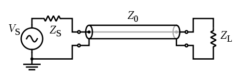
A transmission line drawn as two black wires. At a distance x into the line, there is current phasor I(x) traveling through each wire, and there is a voltage difference phasor V(x) between the wires (bottom voltage minus top voltage). If ${\displaystyle Z_{0}}$ is the characteristic impedance of the line, then ${\displaystyle V(x)/I(x)=Z_{0}}$ for a wave moving rightward, or ${\displaystyle V(x)/I(x)=-Z_{0}}$ for a wave moving leftward.

Schematic representation of a circuit where a source is coupled to a load with a transmission line having characteristic impedance ${\displaystyle Z_{0}}$

The characteristic impedance or surge impedance (usually written Z₀) of a uniform transmission line is the ratio of the amplitudes of voltage and current of a wave travelling in one direction along the line in the absence of reflections in the other direction. Equivalently, it can be defined as the input impedance of a transmission line when its length is infinite. Characteristic impedance is determined by the geometry and materials of the transmission line and, for a uniform line, is not dependent on its length. The SI unit of characteristic impedance is the ohm.

The characteristic impedance of a lossless transmission line is purely real, with no reactive component (see below). Energy supplied by a source at one end of such a line is transmitted through the line without being dissipated in the line itself. A transmission line of finite length (lossless or lossy) that is terminated at one end with an impedance equal to the characteristic impedance appears to the source like an infinitely long transmission line and produces no reflections.

Transmission line model

The characteristic impedance ${\displaystyle Z(\omega )}$ of an infinite transmission line at a given angular frequency ${\displaystyle \omega }$ is the ratio of the voltage and current of a pure sinusoidal wave of the same frequency travelling along the line. This relation is also the case for finite transmission lines until the wave reaches the end of the line. Generally, a wave is reflected back along the line in the opposite direction. When the reflected wave reaches the source, it is reflected yet again, adding to the transmitted wave and changing the ratio of the voltage and current at the input, causing the voltage-current ratio to no longer equal the characteristic impedance. This new ratio including the reflected energy is called the input impedance of that particular transmission line and load.

The input impedance of an infinite line is equal to the characteristic impedance since the transmitted wave is never reflected back from the end. Equivalently: The characteristic impedance of a line is that impedance which, when terminating an arbitrary length of line at its output, produces an input impedance of equal value. This is so because there is no reflection on a line terminated in its own characteristic impedance.

Schematic of Heaviside's model of an infinitesimal segment of transmission line

Applying the transmission line model based on the telegrapher's equations as derived below, ^{[1] [2]} the general expression for the characteristic impedance of a transmission line is: $${\displaystyle Z_{0}={\sqrt {{\frac {R+j\omega L}{G+j\omega C}}\,}}}$$ where

• ${\displaystyle R}$ is the resistance per unit length, considering the two conductors to be in series,
• ${\displaystyle L}$ is the inductance per unit length,
• ${\displaystyle G}$ is the conductance of the dielectric per unit length,
• ${\displaystyle C}$ is the capacitance per unit length,
• ${\displaystyle j}$ is the imaginary unit, and
• ${\displaystyle \omega }$ is the angular frequency.

This expression extends to DC by letting ${\displaystyle \omega }$ tend to 0.

A surge of energy on a finite transmission line will see an impedance of ${\displaystyle Z_{0}}$ prior to any reflections returning; hence surge impedance is an alternative name for characteristic impedance. Although an infinite line is assumed, since all quantities are per unit length, the “per length” parts of all the units cancel, and the characteristic impedance is independent of the length of the transmission line.

The voltage and current phasors on the line are related by the characteristic impedance as: $${\displaystyle Z_{\text{0}}={\frac {V_{(+)}}{I_{(+)}}}=-{\frac {V_{(-)}}{I_{(-)}}}}$$ where the subscripts (+) and (−) mark the separate constants for the waves traveling forward (+) and backward (−). The rightmost expression has a negative sign because the current in the backward wave has the opposite direction to current in the forward wave.

Derivation

Using the telegrapher's equation

Main article: telegrapher's equation

Consider one section of the transmission line for the derivation of the characteristic impedance. The voltage on the left would be ${\displaystyle \ V\ }$ and on the right side would be ${\displaystyle \ V+\operatorname {d} V~.}$ This figure is to be used for both the derivation methods.

The differential equations describing the dependence of the voltage and current on time and space are linear, so that a linear combination of solutions is again a solution. This means that we can consider solutions with a time dependence ${\displaystyle \ e^{j\omega t}\$ ;} doing so is functionally equivalent of solving for the Fourier coefficients for voltage and current amplitudes, at some fixed angular frequency ${\displaystyle \ \omega ~.}$ Doing so causes the time dependence to factor out, leaving an ordinary differential equation for the coefficients, which will be phasors, dependent on position (space) only. Moreover, the parameters can be generalized to be frequency-dependent. ^[1]

Let $${\displaystyle V(x,t)\equiv V(x)\ e^{+j\omega t}}$$ and $${\displaystyle I(x,t)\equiv I(x)\ e^{+j\omega t}}$$

Take the positive direction for ${\displaystyle \ V\ }$ and ${\displaystyle \ I\ }$ in the loop to be clockwise.

We find that $${\displaystyle \ \operatorname {d} V=-\left(R+j\ \omega L\right)I\ \operatorname {d} x=-Z'\ I\ \operatorname {d} x}$$ and $${\displaystyle \ \operatorname {d} I=-\left(G+j\ \omega C\right)V\ \operatorname {d} x=-Y'\ V\ \operatorname {d} x}$$ or $${\displaystyle \ {\frac {\ \operatorname {d} V\ }{\ \operatorname {d} x\ }}=-Z'\ I\qquad {\text{ and }}\qquad {\frac {\ \operatorname {d} I\ }{\ \operatorname {d} x\ }}=-Y'\ V}$$ where $${\displaystyle \ Z'\equiv R+j\ \omega L\qquad {\text{ and }}\qquad Y'\equiv G+j\ \omega C~.}$$

These two first-order equations are easily uncoupled by a second differentiation, with the results: $${\displaystyle \ {\frac {\ \operatorname {d} ^{2}V\ }{\ \operatorname {d} x^{2}}}=Z'Y'\ V\ }$$ and $${\displaystyle \ {\frac {\ \operatorname {d} ^{2}I\ }{\ \operatorname {d} x^{2}}}=Z'Y'\ I\ }$$

Notice that both ${\displaystyle \ V\ }$ and ${\displaystyle \ I\ }$ satisfy the same equation.

Since ${\displaystyle \ Z'Y'\ }$ is independent of ${\displaystyle \ x\ }$ and ${\displaystyle \ t\ ,}$ it can be represented by a single constant ${\displaystyle \ -k^{2}~.}$ (The minus sign is included for later convenience.) That is: $${\displaystyle \ -k^{2}\equiv Z'\,Y'\ }$$ so $${\displaystyle \ jk=\pm {\sqrt {Z'\,Y'\ }}\ }$$

We can write the above equation as $${\displaystyle \ k=\pm \omega {\sqrt {\left(L-j\ {\frac {\ R\ }{\omega }}\right)\left(C-j\ {\frac {\ G\ }{\omega }}\right)\ }}=\pm \omega {\sqrt {L\ C\ }}{\sqrt {\left(1-j\ {\frac {R}{\ \omega L\ }}\right)\left(1-j\ {\frac {G}{\ \omega C\ }}\right)\ }}\ }$$ which is correct for any transmission line in general. And for typical transmission lines, that are carefully built from wire with low loss resistance ${\displaystyle \ R\ }$ and small insulation leakage conductance ${\displaystyle \ G\$ ;} further, used for high frequencies, the inductive reactance ${\displaystyle \ \omega L\ }$ and the capacitive admittance ${\displaystyle \ \omega C\ }$ will both be large, so the constant ${\displaystyle \ k\ }$ is very close to being a real number: $${\displaystyle \ k\approx \pm \omega {\sqrt {LC\;}}~.}$$

With this definition of ${\displaystyle \ k\ ,}$ the position- or ${\displaystyle \ x}$-dependent part will appear as ${\displaystyle \ \pm j\ k\ x\ }$ in the exponential solutions of the equation, similar to the time-dependent part ${\displaystyle \ +j\ \omega \ t\ }$ so the solution reads $${\displaystyle V(x)=v_{(+)}\ e^{-jkx}+v_{(-)}\ e^{+jkx}}$$ where ${\displaystyle \ v_{(+)}\ }$ and ${\displaystyle \ v_{(-)}\ }$ are the constants of integration for the forward moving (+) and backward moving (−) waves, as in the prior section. When we recombine the time-dependent part we obtain the full solution: $${\displaystyle \ V(x,t)~=~V(x)\ e^{+j\omega t}~=~v_{(+)}\ e^{-jkx+j\omega t}+v_{(-)}e^{+jkx+j\omega t}~.}$$

Since the equation for ${\displaystyle \ I\ }$ is the same form, it has a solution of the same form: $${\displaystyle \ I(x)=i_{(+)}\ e^{-jkx}+i_{(-)}\ e^{+jkx}\ ,}$$ where ${\displaystyle \ i_{(+)}\ }$ and ${\displaystyle \ i_{(-)}\ }$ are again constants of integration.

The above equations are the wave solution for ${\displaystyle V}$ and ${\displaystyle I}$. In order to be compatible, they must still satisfy the original differential equations, one of which is $${\displaystyle \ {\frac {\ \operatorname {d} V\ }{\ \operatorname {d} x\ }}=-Z'I~.}$$

Substituting the solutions for ${\displaystyle \ V\ }$ and ${\displaystyle \ I\ }$ into the above equation, we get $${\displaystyle \ {\frac {\operatorname {d} }{\ \operatorname {d} x\ }}\left[v_{(+)}\ e^{-j\ k\ x}+v_{(-)}\ e^{+j\ k\ x}\right]=-(R+j\ \omega L)\left[\ i_{(+)}\ e^{-j\ k\ x}+i_{(-)}\ e^{+j\ k\ x}\right]}$$ or $${\displaystyle \ -j\ k\ v_{(+)}\ e^{-j\ k\ x}+jk\ v_{(-)}\ e^{+j\ k\ x}=-(R+j\omega L)\ i_{(+)}\ e^{-jkx}-\left(R+j\ \omega L\right)\ i_{(-)}\ e^{+jkx}}$$

Isolating distinct powers of ${\displaystyle \ e\ }$ and combining identical powers, we see that in order for the above equation to hold for all possible values of ${\displaystyle \ x\ }$ we must have:

For the co-efficients of ${\displaystyle \ e^{-j\ k\ x}\ }$: $${\displaystyle \ -j\ k\ v_{(+)}=-\left(R+j\ \omega L\right)\ i_{(+)}\ }$$

For the co-efficients of ${\displaystyle \ e^{+j\ k\ x}\ }$: $${\displaystyle \ +j\ k\ v_{(-)}=-\left(R+j\ \omega L\right)\ i_{(-)}\ }$$

Since ${\textstyle \ j\ k={\sqrt {\left(R+j\ \omega L\right)\left(G+j\ \omega C\right)\ }}\ }$$${\displaystyle \ {\begin{aligned}+{\frac {v_{(+)}}{i_{(+)}}}&={\frac {\ R+j\ \omega L\ }{j\ k}}={\sqrt {{\frac {\ R+j\ \omega L\ }{G+j\ \omega C}}\ }}\equiv Z_{0}\\[1ex]-{\frac {v_{(-)}}{i_{(-)}}}&={\frac {\ R+j\ \omega L\ }{j\ k}}={\sqrt {{\frac {\ R+j\ \omega L\ }{G+j\ \omega C}}\ }}\equiv Z_{0}\end{aligned}}\ }$$ hence, for valid solutions require $${\displaystyle \ v_{(+)}=+Z_{0}\ i_{(+)}\quad {\text{ and }}\quad v_{(-)}=-Z_{0}\ i_{(-)}\ }$$

It can be seen that the constant ${\displaystyle \ Z_{0}\ ,}$ defined in the above equations has the dimensions of impedance (ratio of voltage to current) and is a function of primary constants of the line and operating frequency. It is called the “characteristic impedance” of the transmission line, and conventionally denoted by ${\displaystyle \ Z_{0}~.}$ ^[2] $${\displaystyle Z_{0}\quad =\quad {\sqrt {{\frac {\ R+j\ \omega L\ }{G+j\ \omega C}}\ }}\quad =\quad {\sqrt {\ {\frac {\ L\ }{C}}\ }}{\sqrt {{\frac {\ 1-j\ \left({\frac {R}{\ \omega L\ }}\right)\,}{\ 1-j\ \left({\frac {G}{\ \omega C\ }}\right)\ }}\ }}}$$ which holds generally, for any transmission line. For well-functioning transmission lines, with either ${\displaystyle \ R\ }$ and ${\displaystyle \ G\ }$ both very small, or with ${\displaystyle \ \omega \ }$ very high, or all of the above, we get $${\displaystyle Z_{0}\approx {\sqrt {{\frac {\ L\ }{C}}\ }}}$$ hence the characteristic impedance is typically very close to being a real number. Manufacturers make commercial cables to approximate this condition very closely over a wide range of frequencies.

As a limiting case of infinite ladder networks

Intuition

See also: Iterative impedance and Constant k filters

Iterative impedance of an infinite ladder of L-circuit sections

Iterative impedance of the equivalent finite L-circuit

Consider an infinite ladder network consisting of a series impedance ${\displaystyle \ Z\ }$ and a shunt admittance ${\displaystyle \ Y~.}$ Let its input impedance be ${\displaystyle \ Z_{\mathrm {IT} }~.}$ If a new pair of impedance ${\displaystyle \ Z\ }$ and admittance ${\displaystyle \ Y\ }$ is added in front of the network, its input impedance ${\displaystyle \ Z_{\mathrm {IT} }\ }$ remains unchanged since the network is infinite. Thus, it can be reduced to a finite network with one series impedance ${\displaystyle \ Z\ }$ and two parallel impedances ${\displaystyle \ 1/Y\ }$ and ${\displaystyle \ Z_{\text{IT}}~.}$ Its input impedance is given by the expression ^{[3] [4] [5]}

${\displaystyle \ Z_{\mathrm {IT} }=Z+\left({\frac {\ 1\ }{Y}}\parallel Z_{\mathrm {IT} }\right)\ }$

which is also known as its iterative impedance. Its solution is:

${\displaystyle \ Z_{\mathrm {IT} }={Z \over 2}\pm {\sqrt {{Z^{2} \over 4}+{Z \over Y}}}\ }$

For a transmission line, it can be seen as a limiting case of an infinite ladder network with infinitesimal impedance and admittance at a constant ratio. ^{[6] [4] [5]} Taking the positive root, this equation simplifies to:

${\displaystyle \ Z_{\mathrm {IT} }={\sqrt {{\frac {\ Z\ }{Y}}\ }}\ }$

Derivation

Using this insight, many similar derivations exist in several books ^{[6] [4] [5]} and are applicable to both lossless and lossy lines. ^[7]

Here, we follow an approach posted by Tim Healy. ^[8] The line is modeled by a series of differential segments with differential series elements ${\displaystyle \ \left(R\ \operatorname {d} x,\ L\ \operatorname {d} x\right)\ }$ and shunt elements ${\displaystyle \ \left(C\ \operatorname {d} x,\ G\ \operatorname {d} x\ \right)\ }$ (as shown in the figure at the beginning of the article). The characteristic impedance is defined as the ratio of the input voltage to the input current of a semi-infinite length of line. We call this impedance ${\displaystyle \ Z_{0}~.}$ That is, the impedance looking into the line on the left is ${\displaystyle \ Z_{0}~.}$ But, of course, if we go down the line one differential length ${\displaystyle \ \operatorname {d} x\ ,}$ the impedance into the line is still ${\displaystyle \ Z_{0}~.}$ Hence we can say that the impedance looking into the line on the far left is equal to ${\displaystyle \ Z_{0}\ }$ in parallel with ${\displaystyle \ C\ \operatorname {d} x\ }$ and ${\displaystyle \ G\ \operatorname {d} x\ ,}$ all of which is in series with ${\displaystyle \ R\ \operatorname {d} x\ }$ and ${\displaystyle \ L\ \operatorname {d} x~.}$ Hence: $${\displaystyle {\begin{aligned}Z_{0}&=(R+j\ \omega L)\ \operatorname {d} x+{\frac {1}{\ (G+j\omega C)\ \operatorname {d} x+{\frac {1}{\ Z_{0}\ }}\ }}\\[1ex]Z_{0}&=(R+j\ \omega L)\ \operatorname {d} x+{\frac {\ Z_{0}\ }{Z_{0}\ (G+j\omega C)\ \operatorname {d} x+1\,}}\\[1ex]Z_{0}+Z_{0}^{2}\ (G+j\ \omega C)\ \operatorname {d} x&=(R+j\ \omega L)\ \operatorname {d} x+Z_{0}\ (G+j\ \omega C)\ \operatorname {d} x\ (R+j\ \omega L)\ \operatorname {d} x+Z_{0}\end{aligned}}}$$

The added ${\displaystyle \ Z_{0}\ }$ terms cancel, leaving $${\displaystyle \ Z_{0}^{2}\ (G+j\ \omega C)\ \operatorname {d} x=\left(R+j\ \omega L\right)\ \operatorname {d} x+Z_{0}\ \left(G+j\ \omega C\right)\ \left(R+j\ \omega L\right)\ \left(\operatorname {d} x\right)^{2}}$$

The first-power ${\displaystyle \ \operatorname {d} x\ }$ terms are the highest remaining order. Dividing out the common factor of ${\displaystyle \ \operatorname {d} x\ ,}$ and dividing through by the factor ${\displaystyle \ \left(G+j\ \omega C\right)\ ,}$ we get $${\displaystyle \ Z_{0}^{2}={\frac {\left(R+j\ \omega L\right)}{\ \left(G+j\ \omega C\right)\ }}+Z_{0}\ \left(R+j\ \omega L\right)\ \operatorname {d} x~.}$$

In comparison to the factors whose ${\displaystyle \ \operatorname {d} x\ }$ divided out, the last term, which still carries a remaining factor ${\displaystyle \ \operatorname {d} x\ ,}$ is infinitesimal relative to the other, now finite terms, so we can drop it. That leads to $${\displaystyle \ Z_{0}=\pm {\sqrt {{\frac {\ R+j\ \omega L\ }{G+j\ \omega C}}\ }}~.}$$

Reversing the sign ± applied to the square root has the effect of reversing the direction of the flow of current.

Lossless line

The analysis of lossless lines provides an accurate approximation for real transmission lines that simplifies the mathematics considered in modeling transmission lines. A lossless line is defined as a transmission line that has no line resistance and no dielectric loss. This would imply that the conductors act like perfect conductors and the dielectric acts like a perfect dielectric. For a lossless line, R and G are both zero, so the equation for characteristic impedance derived above reduces to: $${\displaystyle Z_{0}={\sqrt {{\frac {L}{C}}\,}}\,.}$$

In particular, ${\displaystyle Z_{0}}$ does not depend any more upon the frequency. The above expression is wholly real, since the imaginary term j has canceled out, implying that ${\displaystyle Z_{0}}$ is purely resistive. For a lossless line terminated in ${\displaystyle Z_{0}}$, there is no loss of current across the line, and so the voltage remains the same along the line. The lossless line model is a useful approximation for many practical cases, such as low-loss transmission lines and transmission lines with high frequency. For both of these cases, R and G are much smaller than ωL and ωC, respectively, and can thus be ignored.

The solutions to the long line transmission equations include incident and reflected portions of the voltage and current: $${\displaystyle {\begin{aligned}V&={\frac {V_{r}+I_{r}Z_{c}}{2}}e^{\gamma x}+{\frac {V_{r}-I_{r}Z_{c}}{2}}e^{-\gamma x}\\[1ex]I&={\frac {V_{r}/Z_{c}+I_{r}}{2}}e^{\gamma x}-{\frac {V_{r}/Z_{c}-I_{r}}{2}}e^{-\gamma x}\end{aligned}}}$$ When the line is terminated with its characteristic impedance, the reflected portions of these equations are reduced to 0 and the solutions to the voltage and current along the transmission line are wholly incident. Without a reflection of the wave, the load that is being supplied by the line effectively blends into the line making it appear to be an infinite line. In a lossless line this implies that the voltage and current remain the same everywhere along the transmission line. Their magnitudes remain constant along the length of the line and are only rotated by a phase angle.

Surge impedance loading

In electric power transmission, the characteristic impedance of a transmission line is expressed in terms of the surge impedance loading (SIL), or natural loading, being the power loading at which reactive power is neither produced nor absorbed: $${\displaystyle {\mathit {SIL}}={\frac {{V_{\mathrm {LL} }}^{2}}{Z_{0}}}}$$ in which ${\displaystyle V_{\mathrm {LL} }}$ is the RMS line-to-line voltage in volts.

Loaded below its SIL, the voltage at the load will be greater than the system voltage. Above it, the load voltage is depressed. The Ferranti effect describes the voltage gain towards the remote end of a very lightly loaded (or open ended) transmission line. Underground cables normally have a very low characteristic impedance, resulting in an SIL that is typically in excess of the thermal limit of the cable.

Practical examples

Standard	Impedance (Ω)	Tolerance
Category 5	100	±5Ω [9]
USB	90	±15% [10]
HDMI	95	±15% [11]
IEEE 1394	108	+3% −2% [12]
VGA	75	±5% [13]
DisplayPort	100	±20% [11]
DVI	95	±15% [11]
PCIe	85	±15% [11]
Overhead power line	400	Typical [14]
Underground power line	40	Typical [14]

The characteristic impedance of coaxial cables (coax) is commonly chosen to be 50 Ω for RF and microwave applications. Coax for video applications is usually 75 Ω for its lower loss.

See also: Nominal impedance § 50 Ω and 75 Ω

See also

• Ampère's circuital law  – Concept in classical electromagnetism
• Characteristic acoustic impedance  – Opposition that a system presents to an acoustic pressurePages displaying short descriptions of redirect targets
• Iterative impedance, characteristic impedance is a limiting case of this
• Maxwell's equations  – Equations describing classical electromagnetism
• Wave impedance  – Constant related to electromagnetic wave propagation in a medium
• Space cloth  – Hypothetical plane with resistivity of 376.7 ohms per square.

References

1. "The Telegrapher's Equation". mysite.du.edu. Retrieved 9 September 2018.
2. "Derivation of Characteristic Impedance of Transmission line". GATE ECE 2018. 16 April 2016. Archived from the original on 9 September 2018. Retrieved 9 September 2018.
3. Feynman, Richard; Leighton, Robert B.; Sands, Matthew. "Section 22-6. A ladder network". The Feynman Lectures on Physics. Vol. 2.
4. Lee, Thomas H. (2004). "2.5 Driving-point impedance of iterated structure". Planar Microwave Engineering: A practical guide to theory, measurement, and circuits. Cambridge University Press. p. 44.
5. Niknejad, Ali M. (2007). "Section 9.2. An infinite ladder network". Electromagnetics for high-speed analog and digital communication circuits.
6. Feynman, Richard; Leighton, Robert B.; Sands, Matthew. "Section 22-7. Filter". The Feynman Lectures on Physics. Vol. 2. If we imagine the line as broken up into small lengths Δℓ, each length will look like one section of the L-C ladder with a series inductance ΔL and a shunt capacitance ΔC. We can then use our results for the ladder filter. If we take the limit as Δℓ goes to zero, we have a good description of the transmission line. Notice that as Δℓ is made smaller and smaller, both ΔL and ΔC decrease, but in the same proportion, so that the ratio ΔL/ΔC remains constant. So if we take the limit of Eq. (22.28) as ΔL and ΔC go to zero, we find that the characteristic impedance z0 is a pure resistance whose magnitude is √(ΔL/ΔC). We can also write the ratio ΔL/ΔC as L0/C0, where L0 and C0 are the inductance and capacitance of a unit length of the line; then we have ${\displaystyle {\sqrt {\frac {L_{0}}{C_{0}}}}}$.
7. Lee, Thomas H. (2004). "2.6.2. Characteristic impedance of a lossy transmission line". Planar Microwave Engineering: A practical guide to theory, measurement, and circuits. Cambridge University Press. p. 47.
8. "Characteristic impedance". ee.scu.edu. Archived from the original on 2017-05-19. Retrieved 2018-09-09.
9. "SuperCat OUTDOOR CAT 5e U/UTP" (PDF). Archived from the original (PDF) on 2012-03-16.
10. "Chapter 2 – Hardware". USB in a NutShell. Beyond Logic.org. Retrieved 2007-08-25.
11. "AN10798 DisplayPort PCB layout guidelines" (PDF). Archived (PDF) from the original on 2022-10-09. Retrieved 2019-12-29.
12. "Evaluation" (PDF). materias.fi.uba.ar. Archived (PDF) from the original on 2022-10-09. Retrieved 2019-12-29.
13. "VMM5FL" (PDF). pro video data sheets. Archived from the original (PDF) on 2016-04-02. Retrieved 2016-03-21.
14. Singh 2008, p. 212.

Sources

• Guile, A.E. (1977). Electrical Power Systems. ISBN   0-08-021729-X.
• Pozar, D.M. (February 2004). Microwave Engineering (3rd ed.). ISBN   0-471-44878-8.
• Ulaby, F.T. (2004). Fundamentals of Applied Electromagnetics (media ed.). Prentice Hall. ISBN   0-13-185089-X.
• Singh, S. N. (23 June 2008). Electric Power Generation: Transmission and Distribution (2 ed.). PHI Learning Pvt. Ltd. p. 212. ISBN   9788120335608. OCLC   1223330325.

External links

 This article incorporates public domain material from Federal Standard 1037C. General Services Administration. Archived from the original on 2022-01-22.