
Principal component analysis (PCA) is a linear dimensionality reduction technique with applications in exploratory data analysis, visualization and data preprocessing.
In signal processing, independent component analysis (ICA) is a computational method for separating a multivariate signal into additive subcomponents. This is done by assuming that at most one subcomponent is Gaussian and that the subcomponents are statistically independent from each other. ICA was invented by Jeanny Hérault and Christian Jutten in 1985. ICA is a special case of blind source separation. A common example application of ICA is the "cocktail party problem" of listening in on one person's speech in a noisy room.

An event-related potential (ERP) is the measured brain response that is the direct result of a specific sensory, cognitive, or motor event. More formally, it is any stereotyped electrophysiological response to a stimulus. The study of the brain in this way provides a noninvasive means of evaluating brain functioning.

Synthetic-aperture radar (SAR) is a form of radar that is used to create two-dimensional images or three-dimensional reconstructions of objects, such as landscapes. SAR uses the motion of the radar antenna over a target region to provide finer spatial resolution than conventional stationary beam-scanning radars. SAR is typically mounted on a moving platform, such as an aircraft or spacecraft, and has its origins in an advanced form of side looking airborne radar (SLAR). The distance the SAR device travels over a target during the period when the target scene is illuminated creates the large synthetic antenna aperture. Typically, the larger the aperture, the higher the image resolution will be, regardless of whether the aperture is physical or synthetic – this allows SAR to create high-resolution images with comparatively small physical antennas. For a fixed antenna size and orientation, objects which are further away remain illuminated longer – therefore SAR has the property of creating larger synthetic apertures for more distant objects, which results in a consistent spatial resolution over a range of viewing distances.
In signal processing, time–frequency analysis comprises those techniques that study a signal in both the time and frequency domains simultaneously, using various time–frequency representations. Rather than viewing a 1-dimensional signal and some transform, time–frequency analysis studies a two-dimensional signal – a function whose domain is the two-dimensional real plane, obtained from the signal via a time–frequency transform.
In statistics, a mixture model is a probabilistic model for representing the presence of subpopulations within an overall population, without requiring that an observed data set should identify the sub-population to which an individual observation belongs. Formally a mixture model corresponds to the mixture distribution that represents the probability distribution of observations in the overall population. However, while problems associated with "mixture distributions" relate to deriving the properties of the overall population from those of the sub-populations, "mixture models" are used to make statistical inferences about the properties of the sub-populations given only observations on the pooled population, without sub-population identity information. Mixture models are used for clustering, under the name model-based clustering, and also for density estimation.
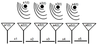
Array processing is a wide area of research in the field of signal processing that extends from the simplest form of 1 dimensional line arrays to 2 and 3 dimensional array geometries. Array structure can be defined as a set of sensors that are spatially separated, e.g. radio antenna and seismic arrays. The sensors used for a specific problem may vary widely, for example microphones, accelerometers and telescopes. However, many similarities exist, the most fundamental of which may be an assumption of wave propagation. Wave propagation means there is a systemic relationship between the signal received on spatially separated sensors. By creating a physical model of the wave propagation, or in machine learning applications a training data set, the relationships between the signals received on spatially separated sensors can be leveraged for many applications.
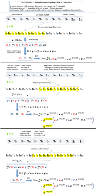
In signal processing, a filter bank is an array of bandpass filters that separates the input signal into multiple components, each one carrying a sub-band of the original signal. One application of a filter bank is a graphic equalizer, which can attenuate the components differently and recombine them into a modified version of the original signal. The process of decomposition performed by the filter bank is called analysis ; the output of analysis is referred to as a subband signal with as many subbands as there are filters in the filter bank. The reconstruction process is called synthesis, meaning reconstitution of a complete signal resulting from the filtering process.
Linear discriminant analysis (LDA), normal discriminant analysis (NDA), or discriminant function analysis is a generalization of Fisher's linear discriminant, a method used in statistics and other fields, to find a linear combination of features that characterizes or separates two or more classes of objects or events. The resulting combination may be used as a linear classifier, or, more commonly, for dimensionality reduction before later classification.
k-means clustering is a method of vector quantization, originally from signal processing, that aims to partition n observations into k clusters in which each observation belongs to the cluster with the nearest mean, serving as a prototype of the cluster. This results in a partitioning of the data space into Voronoi cells. k-means clustering minimizes within-cluster variances, but not regular Euclidean distances, which would be the more difficult Weber problem: the mean optimizes squared errors, whereas only the geometric median minimizes Euclidean distances. For instance, better Euclidean solutions can be found using k-medians and k-medoids.
Non-negative matrix factorization, also non-negative matrix approximation is a group of algorithms in multivariate analysis and linear algebra where a matrix V is factorized into (usually) two matrices W and H, with the property that all three matrices have no negative elements. This non-negativity makes the resulting matrices easier to inspect. Also, in applications such as processing of audio spectrograms or muscular activity, non-negativity is inherent to the data being considered. Since the problem is not exactly solvable in general, it is commonly approximated numerically.
Computational auditory scene analysis (CASA) is the study of auditory scene analysis by computational means. In essence, CASA systems are "machine listening" systems that aim to separate mixtures of sound sources in the same way that human listeners do. CASA differs from the field of blind signal separation in that it is based on the mechanisms of the human auditory system, and thus uses no more than two microphone recordings of an acoustic environment. It is related to the cocktail party problem.
In statistical signal processing, the goal of spectral density estimation (SDE) or simply spectral estimation is to estimate the spectral density of a signal from a sequence of time samples of the signal. Intuitively speaking, the spectral density characterizes the frequency content of the signal. One purpose of estimating the spectral density is to detect any periodicities in the data, by observing peaks at the frequencies corresponding to these periodicities.

In time series analysis, singular spectrum analysis (SSA) is a nonparametric spectral estimation method. It combines elements of classical time series analysis, multivariate statistics, multivariate geometry, dynamical systems and signal processing. Its roots lie in the classical Karhunen (1946)–Loève spectral decomposition of time series and random fields and in the Mañé (1981)–Takens (1981) embedding theorem. SSA can be an aid in the decomposition of time series into a sum of components, each having a meaningful interpretation. The name "singular spectrum analysis" relates to the spectrum of eigenvalues in a singular value decomposition of a covariance matrix, and not directly to a frequency domain decomposition.
Stationary Subspace Analysis (SSA) in statistics is a blind source separation algorithm which factorizes a multivariate time series into stationary and non-stationary components.
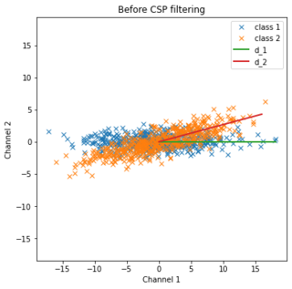
Common spatial pattern (CSP) is a mathematical procedure used in signal processing for separating a multivariate signal into additive subcomponents which have maximum differences in variance between two windows.
Joint Approximation Diagonalization of Eigen-matrices (JADE) is an algorithm for independent component analysis that separates observed mixed signals into latent source signals by exploiting fourth order moments. The fourth order moments are a measure of non-Gaussianity, which is used as a proxy for defining independence between the source signals. The motivation for this measure is that Gaussian distributions possess zero excess kurtosis, and with non-Gaussianity being a canonical assumption of ICA, JADE seeks an orthogonal rotation of the observed mixed vectors to estimate source vectors which possess high values of excess kurtosis.
Sparse dictionary learning is a representation learning method which aims at finding a sparse representation of the input data in the form of a linear combination of basic elements as well as those basic elements themselves. These elements are called atoms and they compose a dictionary. Atoms in the dictionary are not required to be orthogonal, and they may be an over-complete spanning set. This problem setup also allows the dimensionality of the signals being represented to be higher than the one of the signals being observed. The above two properties lead to having seemingly redundant atoms that allow multiple representations of the same signal but also provide an improvement in sparsity and flexibility of the representation.
In signal processing, multidimensional empirical mode decomposition is an extension of the one-dimensional (1-D) EMD algorithm to a signal encompassing multiple dimensions. The Hilbert–Huang empirical mode decomposition (EMD) process decomposes a signal into intrinsic mode functions combined with the Hilbert spectral analysis, known as the Hilbert–Huang transform (HHT). The multidimensional EMD extends the 1-D EMD algorithm into multiple-dimensional signals. This decomposition can be applied to image processing, audio signal processing, and various other multidimensional signals.
Dependent component analysis (DCA) is a blind signal separation (BSS) method and an extension of Independent component analysis (ICA). ICA is the separating of mixed signals to individual signals without knowing anything about source signals. DCA is used to separate mixed signals into individual sets of signals that are dependent on signals within their own set, without knowing anything about the original signals. DCA can be ICA if all sets of signals only contain a single signal within their own set.


