
In statistics, a power law is a functional relationship between two quantities, where a relative change in one quantity results in a relative change in the other quantity proportional to the change raised to a constant exponent: one quantity varies as a power of another. The change is independent of the initial size of those quantities.

Flight dynamics is the science of air vehicle orientation and control in three dimensions. The three critical flight dynamics parameters are the angles of rotation in three dimensions about the vehicle's center of gravity (cg), known as pitch, roll and yaw. These are collectively known as aircraft attitude, often principally relative to the atmospheric frame in normal flight, but also relative to terrain during takeoff or landing, or when operating at low elevation. The concept of attitude is not specific to fixed-wing aircraft, but also extends to rotary aircraft such as helicopters, and dirigibles, where the flight dynamics involved in establishing and controlling attitude are entirely different.
In common usage, wind gradient, more specifically wind speed gradient or wind velocity gradient, or alternatively shear wind, is the vertical component of the gradient of the mean horizontal wind speed in the lower atmosphere. It is the rate of increase of wind strength with unit increase in height above ground level. In metric units, it is often measured in units of meters per second of speed, per kilometer of height (m/s/km), which reduces inverse milliseconds (ms−1), a unit also used for shear rate.

In geometry, an envelope of a planar family of curves is a curve that is tangent to each member of the family at some point, and these points of tangency together form the whole envelope. Classically, a point on the envelope can be thought of as the intersection of two "infinitesimally adjacent" curves, meaning the limit of intersections of nearby curves. This idea can be generalized to an envelope of surfaces in space, and so on to higher dimensions.

In meteorology, the planetary boundary layer (PBL), also known as the atmospheric boundary layer (ABL) or peplosphere, is the lowest part of the atmosphere and its behaviour is directly influenced by its contact with a planetary surface. On Earth it usually responds to changes in surface radiative forcing in an hour or less. In this layer physical quantities such as flow velocity, temperature, and moisture display rapid fluctuations (turbulence) and vertical mixing is strong. Above the PBL is the "free atmosphere", where the wind is approximately geostrophic, while within the PBL the wind is affected by surface drag and turns across the isobars.

Microstrip is a type of electrical transmission line which can be fabricated with any technology where a conductor is separated from a ground plane by a dielectric layer known as "substrate". Microstrip lines are used to convey microwave-frequency signals.

Roughness length is a parameter of some vertical wind profile equations that model the horizontal mean wind speed near the ground. In the log wind profile, it is equivalent to the height at which the wind speed theoretically becomes zero in the absence of wind-slowing obstacles and under neutral conditions. In reality, the wind at this height no longer follows a mathematical logarithm. It is so named because it is typically related to the height of terrain roughness elements. For instance, forests tend to have much larger roughness lengths than tundra. The roughness length does not exactly correspond to any physical length. However, it can be considered as a length-scale representation of the roughness of the surface.
The log wind profile is a semi-empirical relationship commonly used to describe the vertical distribution of horizontal mean wind speeds within the lowest portion of the planetary boundary layer. The relationship is well described in the literature.
In fluid mechanics, potential vorticity (PV) is a quantity which is proportional to the dot product of vorticity and stratification. This quantity, following a parcel of air or water, can only be changed by diabatic or frictional processes. It is a useful concept for understanding the generation of vorticity in cyclogenesis, especially along the polar front, and in analyzing flow in the ocean.
In fluid dynamics, the von Kármán constant, named for Theodore von Kármán, is a dimensionless constant involved in the logarithmic law describing the distribution of the longitudinal velocity in the wall-normal direction of a turbulent fluid flow near a boundary with a no-slip condition. The equation for such boundary layer flow profiles is:

Wind engineering is a subset of mechanical engineering, structural engineering, meteorology, and applied physics that analyzes the effects of wind in the natural and the built environment and studies the possible damage, inconvenience or benefits which may result from wind. In the field of engineering it includes strong winds, which may cause discomfort, as well as extreme winds, such as in a tornado, hurricane or heavy storm, which may cause widespread destruction. In the fields of wind energy and air pollution it also includes low and moderate winds as these are relevant to electricity production and dispersion of contaminants.
The Orr–Sommerfeld equation, in fluid dynamics, is an eigenvalue equation describing the linear two-dimensional modes of disturbance to a viscous parallel flow. The solution to the Navier–Stokes equations for a parallel, laminar flow can become unstable if certain conditions on the flow are satisfied, and the Orr–Sommerfeld equation determines precisely what the conditions for hydrodynamic stability are.
Atmospheric tides are global-scale periodic oscillations of the atmosphere. In many ways they are analogous to ocean tides. They can be excited by:
The Penman-Monteith equation approximates net evapotranspiration (ET) from meteorological data as a replacement for direct measurement of evapotranspiration. The equation is widely used, and was derived by the United Nations Food and Agriculture Organization for modeling reference evapotranspiration ET0.
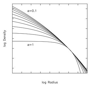
The Einasto profile is a mathematical function that describes how the density of a spherical stellar system varies with distance from its center. Jaan Einasto introduced his model at a 1963 conference in Alma-Ata, Kazakhstan.
A wind erosion equation is an equation used to design wind erosion control systems, which considers soil erodibility, soil roughness, climate, the unsheltered distance across a field, and the vegetative cover on the ground.
Monin–Obukhov (M–O) similarity theory describes the non-dimensionalized mean flow and mean temperature in the surface layer under non-neutral conditions as a function of the dimensionless height parameter, named after Russian scientists A. S. Monin and A. M. Obukhov. Similarity theory is an empirical method that describes universal relationships between non-dimensionalized variables of fluids based on the Buckingham π theorem. Similarity theory is extensively used in boundary layer meteorology since relations in turbulent processes are not always resolvable from first principles.
In physical oceanography and fluid mechanics, the Miles-Phillips mechanism describes the generation of wind waves from a flat sea surface by two distinct mechanisms. Wind blowing over the surface generates tiny wavelets. These wavelets develop over time and become ocean surface waves by absorbing the energy transferred from the wind. The Miles-Phillips mechanism is a physical interpretation of these wind-generated surface waves.
Both mechanisms are applied to gravity-capillary waves and have in common that waves are generated by a resonance phenomenon. The Miles mechanism is based on the hypothesis that waves arise as an instability of the sea-atmosphere system. The Phillips mechanism assumes that turbulent eddies in the atmospheric boundary layer induce pressure fluctuations at the sea surface. The Phillips mechanism is generally assumed to be important in the first stages of wave growth, whereas the Miles mechanism is important in later stages where the wave growth becomes exponential in time.
The Izbash formula is a mathematical expression used to calculate the stability of armourstone in flowing water environments.


