
In fluid dynamics, gravity waves are waves in a fluid medium or at the interface between two media when the force of gravity or buoyancy tries to restore equilibrium. An example of such an interface is that between the atmosphere and the ocean, which gives rise to wind waves.
Rossby waves, also known as planetary waves, are a type of inertial wave naturally occurring in rotating fluids. They were first identified by Sweden-born American meteorologist Carl-Gustaf Arvid Rossby in the Earth's atmosphere in 1939. They are observed in the atmospheres and oceans of Earth and other planets, owing to the rotation of Earth or of the planet involved. Atmospheric Rossby waves on Earth are giant meanders in high-altitude winds that have a major influence on weather. These waves are associated with pressure systems and the jet stream. Oceanic Rossby waves move along the thermocline: the boundary between the warm upper layer and the cold deeper part of the ocean.
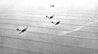
In common usage, wind gradient, more specifically wind speed gradient or wind velocity gradient, or alternatively shear wind, is the vertical component of the gradient of the mean horizontal wind speed in the lower atmosphere. It is the rate of increase of wind strength with unit increase in height above ground level. In metric units, it is often measured in units of meters per second of speed, per kilometer of height (m/s/km), which reduces inverse milliseconds (ms−1), a unit also used for shear rate.
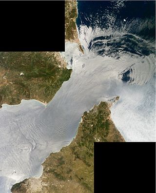
Internal waves are gravity waves that oscillate within a fluid medium, rather than on its surface. To exist, the fluid must be stratified: the density must change with depth/height due to changes, for example, in temperature and/or salinity. If the density changes over a small vertical distance, the waves propagate horizontally like surface waves, but do so at slower speeds as determined by the density difference of the fluid below and above the interface. If the density changes continuously, the waves can propagate vertically as well as horizontally through the fluid.

In meteorology, the planetary boundary layer (PBL), also known as the atmospheric boundary layer (ABL) or peplosphere, is the lowest part of the atmosphere and its behaviour is directly influenced by its contact with a planetary surface. On Earth it usually responds to changes in surface radiative forcing in an hour or less. In this layer physical quantities such as flow velocity, temperature, and moisture display rapid fluctuations (turbulence) and vertical mixing is strong. Above the PBL is the "free atmosphere", where the wind is approximately geostrophic, while within the PBL the wind is affected by surface drag and turns across the isobars.

Roughness length is a parameter of some vertical wind profile equations that model the horizontal mean wind speed near the ground. In the log wind profile, it is equivalent to the height at which the wind speed theoretically becomes zero in the absence of wind-slowing obstacles and under neutral conditions. In reality, the wind at this height no longer follows a mathematical logarithm. It is so named because it is typically related to the height of terrain roughness elements. For instance, forests tend to have much larger roughness lengths than tundra. The roughness length does not exactly correspond to any physical length. However, it can be considered as a length-scale representation of the roughness of the surface.
Surface states are electronic states found at the surface of materials. They are formed due to the sharp transition from solid material that ends with a surface and are found only at the atom layers closest to the surface. The termination of a material with a surface leads to a change of the electronic band structure from the bulk material to the vacuum. In the weakened potential at the surface, new electronic states can be formed, so called surface states.
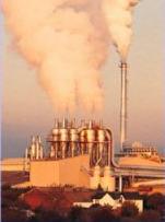
Atmospheric dispersion modeling is the mathematical simulation of how air pollutants disperse in the ambient atmosphere. It is performed with computer programs that include algorithms to solve the mathematical equations that govern the pollutant dispersion. The dispersion models are used to estimate the downwind ambient concentration of air pollutants or toxins emitted from sources such as industrial plants, vehicular traffic or accidental chemical releases. They can also be used to predict future concentrations under specific scenarios. Therefore, they are the dominant type of model used in air quality policy making. They are most useful for pollutants that are dispersed over large distances and that may react in the atmosphere. For pollutants that have a very high spatio-temporal variability and for epidemiological studies statistical land-use regression models are also used.
The wind profile power law is a relationship between the wind speeds at one height, and those at another.
The Obukhov length is used to describe the effects of buoyancy on turbulent flows, particularly in the lower tenth of the atmospheric boundary layer. It was first defined by Alexander Obukhov in 1946. It is also known as the Monin–Obukhov length because of its important role in the similarity theory developed by Monin and Obukhov. A simple definition of the Monin-Obukhov length is that height at which turbulence is generated more by buoyancy than by wind shear.
In fluid mechanics, potential vorticity (PV) is a quantity which is proportional to the dot product of vorticity and stratification. This quantity, following a parcel of air or water, can only be changed by diabatic or frictional processes. It is a useful concept for understanding the generation of vorticity in cyclogenesis, especially along the polar front, and in analyzing flow in the ocean.
The Poisson–Boltzmann equation describes the distribution of the electric potential in solution in the direction normal to a charged surface. This distribution is important to determine how the electrostatic interactions will affect the molecules in solution.
The Debye–Hückel theory was proposed by Peter Debye and Erich Hückel as a theoretical explanation for departures from ideality in solutions of electrolytes and plasmas. It is a linearized Poisson–Boltzmann model, which assumes an extremely simplified model of electrolyte solution but nevertheless gave accurate predictions of mean activity coefficients for ions in dilute solution. The Debye–Hückel equation provides a starting point for modern treatments of non-ideality of electrolyte solutions.
In fluid dynamics, the von Kármán constant, named for Theodore von Kármán, is a dimensionless constant involved in the logarithmic law describing the distribution of the longitudinal velocity in the wall-normal direction of a turbulent fluid flow near a boundary with a no-slip condition. The equation for such boundary layer flow profiles is:
Shear velocity, also called friction velocity, is a form by which a shear stress may be re-written in units of velocity. It is useful as a method in fluid mechanics to compare true velocities, such as the velocity of a flow in a stream, to a velocity that relates shear between layers of flow.
In fluid dynamics, a cnoidal wave is a nonlinear and exact periodic wave solution of the Korteweg–de Vries equation. These solutions are in terms of the Jacobi elliptic function cn, which is why they are coined cnoidal waves. They are used to describe surface gravity waves of fairly long wavelength, as compared to the water depth.
The Eady model is an atmospheric model for baroclinic instability first posed by British meteorologist Eric Eady in 1949 based on his PhD work at Imperial College London.
Monin–Obukhov (M–O) similarity theory describes the non-dimensionalized mean flow and mean temperature in the surface layer under non-neutral conditions as a function of the dimensionless height parameter, named after Russian scientists A. S. Monin and A. M. Obukhov. Similarity theory is an empirical method that describes universal relationships between non-dimensionalized variables of fluids based on the Buckingham π theorem. Similarity theory is extensively used in boundary layer meteorology since relations in turbulent processes are not always resolvable from first principles.
The convective planetary boundary layer (CPBL), also known as the daytime planetary boundary layer, is the part of the lower troposphere most directly affected by solar heating of the Earth's surface.
In physical oceanography and fluid mechanics, the Miles-Phillips mechanism describes the generation of wind waves from a flat sea surface by two distinct mechanisms. Wind blowing over the surface generates tiny wavelets. These wavelets develop over time and become ocean surface waves by absorbing the energy transferred from the wind. The Miles-Phillips mechanism is a physical interpretation of these wind-generated surface waves.
Both mechanisms are applied to gravity-capillary waves and have in common that waves are generated by a resonance phenomenon. The Miles mechanism is based on the hypothesis that waves arise as an instability of the sea-atmosphere system. The Phillips mechanism assumes that turbulent eddies in the atmospheric boundary layer induce pressure fluctuations at the sea surface. The Phillips mechanism is generally assumed to be important in the first stages of wave growth, whereas the Miles mechanism is important in later stages where the wave growth becomes exponential in time.


