Box counting

Last updated

Figure 1. A 32-segment quadric fractal viewed through "boxes" of different sizes. The pattern illustrates self similarity. 32 segment fractal.jpg
Figure 1. A 32-segment quadric fractal viewed through "boxes" of different sizes. The pattern illustrates self similarity.

Box counting is a method of gathering data for analyzing complex patterns by breaking a dataset, object, image, etc. into smaller and smaller pieces, typically "box"-shaped, and analyzing the pieces at each smaller scale. The essence of the process has been compared to zooming in or out using optical or computer based methods to examine how observations of detail change with scale. In box counting, however, rather than changing the magnification or resolution of a lens, the investigator changes the size of the element used to inspect the object or pattern (see Figure 1). Computer based box counting algorithms have been applied to patterns in 1-, 2-, and 3-dimensional spaces. [1] [2] The technique is usually implemented in software for use on patterns extracted from digital media, although the fundamental method can be used to investigate some patterns physically. The technique arose out of and is used in fractal analysis. It also has application in related fields such as lacunarity and multifractal analysis. [3] [4]

Contents

The method

Theoretically, the intent of box counting is to quantify fractal scaling, but from a practical perspective this would require that the scaling be known ahead of time. This can be seen in Figure 1 where choosing boxes of the right relative sizes readily shows how the pattern repeats itself at smaller scales. In fractal analysis, however, the scaling factor is not always known ahead of time, so box counting algorithms attempt to find an optimized way of cutting a pattern up that will reveal the scaling factor. The fundamental method for doing this starts with a set of measuring elements—boxes—consisting of an arbitrary number, called here for convenience, of sizes or calibres, which we will call the set of s. Then these -sized boxes are applied to the pattern and counted. To do this, for each in , a measuring element that is typically a 2-dimensional square or 3-dimensional box with side length corresponding to is used to scan a pattern or data set (e.g., an image or object) according to a predetermined scanning plan to cover the relevant part of the data set, recording, i.e.,counting, for each step in the scan relevant features captured within the measuring element. [3] [4]

Figure 2. The sequence above shows basic steps in extracting a binary contour pattern from an original colour digital image of a neuron. Binarizing neuron image.png
Figure 2. The sequence above shows basic steps in extracting a binary contour pattern from an original colour digital image of a neuron.

The data

The relevant features gathered during box counting depend on the subject being investigated and the type of analysis being done. Two well-studied subjects of box counting, for instance, are binary (meaning having only two colours, usually black and white) [2] and gray-scale [5] digital images (i.e., jpegs, tiffs, etc.). Box counting is generally done on patterns extracted from such still images in which case the raw information recorded is typically based on features of pixels such as a predetermined colour value or range of colours or intensities. When box counting is done to determine a fractal dimension known as the box counting dimension, the information recorded is usually either yes or no as to whether or not the box contained any pixels of the predetermined colour or range (i.e., the number of boxes containing relevant pixels at each is counted). For other types of analysis, the data sought may be the number of pixels that fall within the measuring box, [4] the range or average values of colours or intensities, the spatial arrangement amongst pixels within each box, or properties such as average speed (e.g., from particle flow). [5] [6] [7] [8]

Scan types

Every box counting algorithm has a scanning plan that describes how the data will be gathered, in essence, how the box will be moved over the space containing the pattern. A variety of scanning strategies has been used in box counting algorithms, where a few basic approaches have been modified in order to address issues such as sampling, analysis methods, etc.

Figure 2a. Boxes laid over an image as a fixed grid.
Figure 2b. Boxes slid over an image in an overlapping pattern.
Figure 2c. Boxes laid over an image concentrically focused on each pixel of interest. Fixedstack.gif
Figure 2a. Boxes laid over an image as a fixed grid.
Figure 2b. Boxes slid over an image in an overlapping pattern. Slidestack.gif
Figure 2b. Boxes slid over an image in an overlapping pattern.
Figure 2c. Boxes laid over an image concentrically focused on each pixel of interest. Lcfd.gif
Figure 2c. Boxes laid over an image concentrically focused on each pixel of interest.

Figure 3. Retinal vasculature revealed through box counting analysis; colour-coded local connected fractal dimension analysis done with FracLac freeware for biological image analysis. Retina lcfd.gif
Figure 3. Retinal vasculature revealed through box counting analysis; colour-coded local connected fractal dimension analysis done with FracLac freeware for biological image analysis.

Figure 4. It takes 12 green but 14 yellow boxes to completely cover the black pixels in these identical images. The difference is attributable to the position of the grid, illustrating the importance of grid placement in box counting. Optimal covering grids.png
Figure 4. It takes 12 green but 14 yellow boxes to completely cover the black pixels in these identical images. The difference is attributable to the position of the grid, illustrating the importance of grid placement in box counting.

Fixed grid scans

The traditional approach is to scan in a non-overlapping regular grid or lattice pattern. [3] [4] To illustrate, Figure 2a shows the typical pattern used in software that calculates box counting dimensions from patterns extracted into binary digital images of contours such as the fractal contour illustrated in Figure 1 or the classic example of the coastline of Britain often used to explain the method of finding a box counting dimension. The strategy simulates repeatedly laying a square box as though it were part of a grid overlaid on the image, such that the box for each never overlaps where it has previously been (see Figure 4). This is done until the entire area of interest has been scanned using each and the relevant information has been recorded. [9] [10] When used to find a box counting dimension, the method is modified to find an optimal covering.

Sliding box scans

Another approach that has been used is a sliding box algorithm, in which each box is slid over the image overlapping the previous placement. Figure 2b illustrates the basic pattern of scanning using a sliding box. The fixed grid approach can be seen as a sliding box algorithm with the increments horizontally and vertically equal to . Sliding box algorithms are often used for analyzing textures in lacunarity analysis and have also been applied to multifractal analysis. [2] [8] [11] [12] [13]

Subsampling and local dimensions

Box counting may also be used to determine local variation as opposed to global measures describing an entire pattern. Local variation can be assessed after the data have been gathered and analyzed (e.g., some software colour codes areas according to the fractal dimension for each subsample), but a third approach to box counting is to move the box according to some feature related to the pixels of interest. In local connected dimension box counting algorithms, for instance, the box for each is centred on each pixel of interest, as illustrated in Figure 2c. [7]

Methodological considerations

The implementation of any box counting algorithm has to specify certain details such as how to determine the actual values in , including the minimum and maximum sizes to use and the method of incrementing between sizes. Many such details reflect practical matters such as the size of a digital image but also technical issues related to the specific analysis that will be performed on the data. Another issue that has received considerable attention is how to approximate the so-called "optimal covering" for determining box counting dimensions and assessing multifractal scaling. [5] [14] [15] [16]

Edge effects

One known issue in this respect is deciding what constitutes the edge of the useful information in a digital image, as the limits employed in the box counting strategy can affect the data gathered.

Scaling box size

The algorithm has to specify the type of increment to use between box sizes (e.g., linear vs exponential), which can have a profound effect on the results of a scan.

Grid orientation

As Figure 4 illustrates, the overall positioning of the boxes also influences the results of a box count. One approach in this respect is to scan from multiple orientations and use averaged or optimized data. [17] [18]

To address various methodological considerations, some software is written so users can specify many such details, and some includes methods such as smoothing the data after the fact to be more amenable to the type of analysis being done. [19]

See also

Related Research Articles

Fractal Self similar mathematical structures

In mathematics, a fractal is a self-similar subset of Euclidean space whose fractal dimension strictly exceeds its topological dimension. Fractals appear the same at different levels, as illustrated in successive magnifications of the Mandelbrot set. Fractals exhibit similar patterns at increasingly small scales called self-similarity, also known as expanding symmetry or unfolding symmetry; if this replication is exactly the same at every scale, as in the Menger sponge, it is called affine self-similar. Fractal geometry lies within the mathematical branch of measure theory.

Self-similarity The whole of an object being mathematically similar to part of itself

In mathematics, a self-similar object is exactly or approximately similar to a part of itself. Many objects in the real world, such as coastlines, are statistically self-similar: parts of them show the same statistical properties at many scales. Self-similarity is a typical property of fractals. Scale invariance is an exact form of self-similarity where at any magnification there is a smaller piece of the object that is similar to the whole. For instance, a side of the Koch snowflake is both symmetrical and scale-invariant; it can be continually magnified 3x without changing shape. The non-trivial similarity evident in fractals is distinguished by their fine structure, or detail on arbitrarily small scales. As a counterexample, whereas any portion of a straight line may resemble the whole, further detail is not revealed.

In mathematics, more specifically in fractal geometry, a fractal dimension is a ratio providing a statistical index of complexity comparing how detail in a pattern changes with the scale at which it is measured. It has also been characterized as a measure of the space-filling capacity of a pattern that tells how a fractal scales differently from the space it is embedded in; a fractal dimension does not have to be an integer.

Eigenface

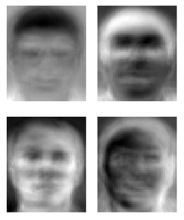
An eigenface is the name given to a set of eigenvectors when used in the computer vision problem of human face recognition. The approach of using eigenfaces for recognition was developed by Sirovich and Kirby (1987) and used by Matthew Turk and Alex Pentland in face classification. The eigenvectors are derived from the covariance matrix of the probability distribution over the high-dimensional vector space of face images. The eigenfaces themselves form a basis set of all images used to construct the covariance matrix. This produces dimension reduction by allowing the smaller set of basis images to represent the original training images. Classification can be achieved by comparing how faces are represented by the basis set.

Image segmentation

In digital image processing and computer vision, image segmentation is the process of partitioning a digital image into multiple segments. The goal of segmentation is to simplify and/or change the representation of an image into something that is more meaningful and easier to analyze. Image segmentation is typically used to locate objects and boundaries in images. More precisely, image segmentation is the process of assigning a label to every pixel in an image such that pixels with the same label share certain characteristics.

Quadtree Tree data structure in which each internal node has exactly four children

A quadtree is a tree data structure in which each internal node has exactly four children. Quadtrees are the two-dimensional analog of octrees and are most often used to partition a two-dimensional space by recursively subdividing it into four quadrants or regions. The data associated with a leaf cell varies by application, but the leaf cell represents a "unit of interesting spatial information".

Minkowski–Bouligand dimension Way of determining the dimension of a fractal set in a Euclidean space by counting the number of fixed-size boxes needed to cover the set as a function of the box size

In fractal geometry, the Minkowski–Bouligand dimension, also known as Minkowski dimension or box-counting dimension, is a way of determining the fractal dimension of a set S in a Euclidean space Rn, or more generally in a metric space (Xd). It is named after the German mathematician Hermann Minkowski and the French mathematician Georges Bouligand.

Hofstadters butterfly A fractal describing the theorised behaviour of electrons in a magnetic field

In condensed matter physics, Hofstadter's butterfly describes the spectral properties of non-interacting two-dimensional electrons in a magnetic field in a lattice. The fractal, self-similar nature of the spectrum was discovered in the 1976 Ph.D. work of Douglas Hofstadter and is one of the early examples of computer graphics. The name reflects the visual resemblance of the figure on the right to a swarm of butterflies flying to infinity.

Multifractal system system with multiple fractal dimensions

A multifractal system is a generalization of a fractal system in which a single exponent is not enough to describe its dynamics; instead, a continuous spectrum of exponents is needed.

Connected-component labeling (CCL), connected-component analysis (CCA), blob extraction, region labeling, blob discovery, or region extraction is an algorithmic application of graph theory, where subsets of connected components are uniquely labeled based on a given heuristic. Connected-component labeling is not to be confused with segmentation.

In stochastic processes, chaos theory and time series analysis, detrended fluctuation analysis (DFA) is a method for determining the statistical self-affinity of a signal. It is useful for analysing time series that appear to be long-memory processes or 1/f noise.

Mean shift is a non-parametric feature-space analysis technique for locating the maxima of a density function, a so-called mode-seeking algorithm. Application domains include cluster analysis in computer vision and image processing.

The Ramer–Douglas–Peucker algorithm, also known as the Douglas–Peucker algorithm and iterative end-point fit algorithm, is an algorithm that decimates a curve composed of line segments to a similar curve with fewer points. It was one of the earliest successful algorithms developed for cartographic generalization.

Fractal analysis is assessing fractal characteristics of data. It consists of several methods to assign a fractal dimension and other fractal characteristics to a dataset which may be a theoretical dataset, or a pattern or signal extracted from phenomena including natural geometric objects, ecology and aquatic sciences, sound, market fluctuations, heart rates, frequency domain in electroencephalography signals, digital images, molecular motion, and data science. Fractal analysis is now widely used in all areas of science. An important limitation of fractal analysis is that arriving at an empirically determined fractal dimension does not necessarily prove that a pattern is fractal; rather, other essential characteristics have to be considered. Fractal analysis is valuable in expanding our knowledge of the structure and function of various systems, and as a potential tool to mathematically assess novel areas of study.

Lacunarity term in geometry and fractal analysis

Lacunarity, from the Latin lacuna, meaning "gap" or "lake", is a specialized term in geometry referring to a measure of how patterns, especially fractals, fill space, where patterns having more or larger gaps generally have higher lacunarity. Beyond being an intuitive measure of gappiness, lacunarity can quantify additional features of patterns such as "rotational invariance" and more generally, heterogeneity. This is illustrated in Figure 1 showing three fractal patterns. When rotated 90°, the first two fairly homogeneous patterns do not appear to change, but the third more heterogeneous figure does change and has correspondingly higher lacunarity. The earliest reference to the term in geometry is usually attributed to Mandelbrot, who, in 1983 or perhaps as early as 1977, introduced it as, in essence, an adjunct to fractal analysis. Lacunarity analysis is now used to characterize patterns in a wide variety of fields and has application in multifractal analysis in particular.

The wavelet transform modulus maxima (WTMM) is a method for detecting the fractal dimension of a signal.

Chaotic scattering is a branch of chaos theory dealing with scattering systems displaying a strong sensitivity to initial conditions. In a classical scattering system there will be one or more impact parameters, b, in which a particle is sent into the scatterer. This gives rise to one or more exit parameters, y, as the particle exits towards infinity. While the particle is traversing the system, there may also be a delay time, T—the time it takes for the particle to exit the system—in addition to the distance travelled, s, which in certain systems, i.e., "billiard-like" systems in which the particle undergoes lossless collisions with hard, fixed objects, the two will be equivalent—see below. In a chaotic scattering system, a minute change in the impact parameter, may give rise to a very large change in the exit parameters.

Robust Principal Component Analysis (RPCA) is a modification of the widely used statistical procedure of principal component analysis (PCA) which works well with respect to grossly corrupted observations. A number of different approaches exist for Robust PCA, including an idealized version of Robust PCA, which aims to recover a low-rank matrix L0 from highly corrupted measurements M = L0 +S0. This decomposition in low-rank and sparse matrices can be achieved by techniques such as Principal Component Pursuit method (PCP), Stable PCP, Quantized PCP, Block based PCP, and Local PCP. Then, optimization methods are used such as the Augmented Lagrange Multiplier Method (ALM), Alternating Direction Method (ADM), Fast Alternating Minimization (FAM), Iteratively Reweighted Least Squares (IRLS ) or alternating projections (AP).

Census transform

The census transform (CT) is an image operator that associates to each pixel of a grayscale image a binary string, encoding whether the pixel has smaller intensity than each of its neighbours, one for each bit. It is a non-parametric transform that depends only on relative ordering of intensities, and not on the actual values of intensity, making it invariant with respect to monotonic variations of illumination, and it behaves well in presence of multimodal distributions of intensity, e.g. along object boundaries. It has applications in computer vision, and it is commonly used in visual correspondence problems such as optical flow calculation and disparity estimation.

Plotting algorithms for the Mandelbrot set Algorithms and methods of plotting the Mandelbrot set on a computing device

There are many programs and algorithms used to plot the Mandelbrot set and other fractals, some of which are described in fractal-generating software. These programs use a variety of algorithms to determine the color of individual pixels efficiently.

References

  1. Liu, Jing Z.; Zhang, Lu D.; Yue, Guang H. (2003). "Fractal Dimension in Human Cerebellum Measured by Magnetic Resonance Imaging". Biophysical Journal. 85 (6): 4041–4046. doi:10.1016/S0006-3495(03)74817-6. PMC   1303704 . PMID   14645092.
  2. 1 2 3 Smith, T. G.; Lange, G. D.; Marks, W. B. (1996). "Fractal methods and results in cellular morphology — dimensions, lacunarity and multifractals". Journal of Neuroscience Methods. 69 (2): 123–136. doi:10.1016/S0165-0270(96)00080-5. PMID   8946315.
  3. 1 2 3 Mandelbrot (1983). The Fractal Geometry of Nature . ISBN   978-0-7167-1186-5.
  4. 1 2 3 4 Iannaccone, Khokha (1996). Fractal Geometry in Biological Systems. p. 143. ISBN   978-0-8493-7636-8.
  5. 1 2 3 Li, J.; Du, Q.; Sun, C. (2009). "An improved box-counting method for image fractal dimension estimation". Pattern Recognition. 42 (11): 2460–2469. doi:10.1016/j.patcog.2009.03.001.
  6. Karperien, Audrey; Jelinek, Herbert F.; Leandro, Jorge de Jesus Gomes; Soares, João V. B.; Cesar Jr, Roberto M.; Luckie, Alan (2008). "Automated detection of proliferative retinopathy in clinical practice". Clinical Ophthalmology (Auckland, N.Z.). 2 (1): 109–122. doi:10.2147/OPTH.S1579. PMC   2698675 . PMID   19668394.
  7. 1 2 Landini, G.; Murray, P. I.; Misson, G. P. (1995). "Local connected fractal dimensions and lacunarity analyses of 60 degrees fluorescein angiograms". Investigative Ophthalmology & Visual Science. 36 (13): 2749–2755. PMID   7499097.
  8. 1 2 Cheng, Qiuming (1997). "Multifractal Modeling and Lacunarity Analysis". Mathematical Geology. 29 (7): 919–932. doi:10.1023/A:1022355723781.
  9. Popescu, D. P.; Flueraru, C.; Mao, Y.; Chang, S.; Sowa, M. G. (2010). "Signal attenuation and box-counting fractal analysis of optical coherence tomography images of arterial tissue". Biomedical Optics Express. 1 (1): 268–277. doi:10.1364/boe.1.000268. PMC   3005165 . PMID   21258464.
  10. King, R. D.; George, A. T.; Jeon, T.; Hynan, L. S.; Youn, T. S.; Kennedy, D. N.; Dickerson, B.; the Alzheimer’s Disease Neuroimaging Initiative (2009). "Characterization of Atrophic Changes in the Cerebral Cortex Using Fractal Dimensional Analysis". Brain Imaging and Behavior. 3 (2): 154–166. doi:10.1007/s11682-008-9057-9. PMC   2927230 . PMID   20740072.
  11. Plotnick, R. E.; Gardner, R. H.; Hargrove, W. W.; Prestegaard, K.; Perlmutter, M. (1996). "Lacunarity analysis: A general technique for the analysis of spatial patterns". Physical Review E. 53 (5): 5461–5468. doi:10.1103/physreve.53.5461. PMID   9964879.
  12. Plotnick, R. E.; Gardner, R. H.; O'Neill, R. V. (1993). "Lacunarity indices as measures of landscape texture". Landscape Ecology. 8 (3): 201–211. doi:10.1007/BF00125351.
  13. McIntyre, N. E.; Wiens, J. A. (2000). "A novel use of the lacunarity index to discern landscape function". Landscape Ecology. 15 (4): 313–321. doi:10.1023/A:1008148514268.
  14. Gorski, A. Z.; Skrzat, J. (2006). "Error estimation of the fractal dimension measurements of cranial sutures". Journal of Anatomy. 208 (3): 353–359. doi:10.1111/j.1469-7580.2006.00529.x. PMC   2100241 . PMID   16533317.
  15. Chhabra, A.; Jensen, R. V. (1989). "Direct determination of the f( alpha ) singularity spectrum". Physical Review Letters. 62 (12): 1327–1330. doi:10.1103/PhysRevLett.62.1327. PMID   10039645.
  16. Fernández, E.; Bolea, J. A.; Ortega, G.; Louis, E. (1999). "Are neurons multifractals?". Journal of Neuroscience Methods. 89 (2): 151–157. doi:10.1016/s0165-0270(99)00066-7. PMID   10491946.
  17. Karperien (2004). Defining Microglial Morphology: Form, Function, and Fractal Dimension. Charles Sturt University, Australia.
  18. Schulze, M. M.; Hutchings, N.; Simpson, T. L. (2008). "The Use of Fractal Analysis and Photometry to Estimate the Accuracy of Bulbar Redness Grading Scales". Investigative Ophthalmology & Visual Science. 49 (4): 1398–1406. doi: 10.1167/iovs.07-1306 . PMID   18385056.
  19. Karperien (2002), Box Counting