A dragon curve is any member of a family of self-similarfractal curves, which can be approximated by recursive methods such as Lindenmayer systems. The dragon curve is probably most commonly thought of as the shape that is generated from repeatedly folding a strip of paper in half, although there are other curves that are called dragon curves that are generated differently.
Recursive construction of the curveRecursive construction of the curve
The Heighway dragon can be constructed from a base line segment by repeatedly replacing each segment by two segments with a right angle and with a rotation of 45° alternatively to the right and to the left:[2]
The first 5 iterations and the 9th
The Heighway dragon is also the limit set of the following iterated function system in the complex plane:
with the initial set of points .
Using pairs of real numbers instead, this is the same as the two functions consisting of
Folding the dragon
The Heighway dragon curve can be constructed by folding a strip of paper, which is how it was originally discovered.[1] Take a strip of paper and fold it in half to the right. Fold it in half again to the right. If the strip was opened out now, unbending each fold to become a 90-degree turn, the turn sequence would be RRL, i.e. the second iteration of the Heighway dragon. Fold the strip in half again to the right, and the turn sequence of the unfolded strip is now RRLRRLL – the third iteration of the Heighway dragon. Continuing folding the strip in half to the right to create further iterations of the Heighway dragon (in practice, the strip becomes too thick to fold sharply after four or five iterations).
The folding patterns of this sequence of paper strips, as sequences of right (R) and left (L) folds, are:
1st iteration: R
2nd iteration: R R L
3rd iteration: R R L R R L L
4th iteration: R R L R R L L R R R L L R L L.
Each iteration can be found by copying the previous iteration, then an R, then a second copy of the previous iteration in reverse order with the L and R letters swapped.[1]
Properties
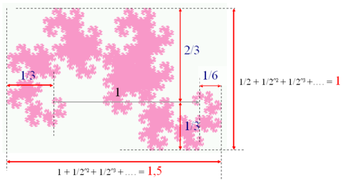
Many self-similarities can be seen in the Heighway dragon curve. The most obvious is the repetition of the same pattern tilted by 45° and with a reduction ratio of . Based on these self-similarities, many of its lengths are simple rational numbers.
Lengths
Self-similarities
Tiling of the plane by dragon curves
The dragon curve can tile the plane. One possible tiling replaces each edge of a square tiling with a dragon curve, using the recursive definition of the dragon starting from a line segment. The initial direction to expand each segment can be determined from a checkerboard coloring of a square tiling, expanding vertical segments into black tiles and out of white tiles, and expanding horizontal segments into white tiles and out of black ones.[3]
As a space-filling curve, the dragon curve has fractal dimension exactly 2. For a dragon curve with initial segment length 1, its area is 1/2, as can be seen from its tilings of the plane.[1]
The boundary of the set covered by the dragon curve has infinite length, with fractal dimension where is the real solution of the equation [4]
Twindragon
Twindragon curve constructed from two Heighway dragons
The twindragon (also known as the Davis–Knuth dragon) can be constructed by placing two Heighway dragon curves back to back. It is also the limit set of the following iterated function system:
where the initial shape is defined by the following set .
It can be also written as a Lindenmayer system – it only needs adding another section in the initial string:
angle 90°
initial string FX+FX+
string rewriting rules
X↦X+YF
Y↦FX−Y.
It is also the locus of points in the complex plane with the same integer part when written in base .[5]
Terdragon
Terdragon curve. A sculpture depicting multiple iterations of the Lindenmayer system that generates the terdragon curve. by Henry Segerman
Having obtained the set of solutions to a linear differential equation, any linear combination of the solutions will, because of the superposition principle, also obey the original equation. In other words, new solutions are obtained by applying a function to the set of existing solutions. This is similar to how an iterated function system produces new points in a set, though not all IFS are linear functions. In a conceptually similar vein, a set of Littlewood polynomials can be arrived at by such iterated applications of a set of functions.
A Littlewood polynomial is a polynomial: where all .
For some we define the following functions:
Starting at z=0 we can generate all Littlewood polynomials of degree d using these functions iteratively d+1 times.[7] For instance:
It can be seen that for , the above pair of functions is equivalent to the IFS formulation of the Heighway dragon. That is, the Heighway dragon, iterated to a certain iteration, describe the set of all Littlewood polynomials up to a certain degree, evaluated at the point . Indeed, when plotting a sufficiently high number of roots of the Littlewood polynomials, structures similar to the dragon curve appear at points close to these coordinates.[7][8][9]
Variants
The dragon curve belongs to a basic set of iteration functions consisting of two lines with four possible orientations at perpendicular angles
Different types of Dragon Curve Variants
Curve
Creators and Creation Year of Dragon Family Members
It is possible to change the turn angle from 90° to other angles. Changing to 120° yields a structure of triangles, while 60° gives the following curve:
A discrete dragon curve can be converted to a dragon polyomino as shown. Like discrete dragon curves, dragon polyominoes approach the fractal dragon curve as a limit.
↑Edgar, Gerald (2008), "Heighway's Dragon", in Edgar, Gerald (ed.), Measure, Topology, and Fractal Geometry, Undergraduate Texts in Mathematics (2nded.), New York: Springer, pp.20–22, doi:10.1007/978-0-387-74749-1, ISBN978-0-387-74748-4, MR2356043
↑Edgar (2008), "Heighway’s Dragon Tiles the Plane", pp. 74–75.
↑Knuth, Donald (1998). "Positional Number Systems". The art of computer programming. Vol. 2 (3rd ed.). Boston: Addison-Wesley. p. 206. ISBN0-201-89684-2. OCLC 48246681.
↑Bernt Wahl; Peter van Roy; Michael Larsen; Eric Kampman (1994). Exploring Fractals on the Machintosh (1sted.). Boston: Addison-Wesley. pp.1–352. ISBN978-0201626308.
This page is based on this Wikipedia article Text is available under the CC BY-SA 4.0 license; additional terms may apply. Images, videos and audio are available under their respective licenses.