Douady rabbit

A Douady rabbit is a fractal derived from the Julia set of the function ${\textstyle f_{c}(z)=z^{2}+c}$, when parameter ${\displaystyle c}$ is near the center of one of the period three bulbs of the Mandelbrot set for a complex quadratic map. It is named after French mathematician Adrien Douady.

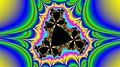
An example of a Douady rabbit. The colors show the number of iterations required to escape.

Background

The Douady rabbit is generated by iterating the Mandelbrot set map ${\displaystyle z_{n+1}=z_{n}^{2}+c}$ on the complex plane, where parameter ${\displaystyle c}$ is fixed to lie in one of the two period three bulb off the main cardioid and ${\displaystyle z}$ ranging over the plane. The resulting image can be colored by corresponding each pixel with a starting value ${\displaystyle z_{0}}$ and calculating the amount of iterations required before the value of ${\displaystyle z_{n}}$ escapes a bounded region, after which it will diverge toward infinity.

It can also be described using the logistic map form of the complex quadratic map, specifically

${\displaystyle z_{n+1}={\mathcal {M}}z_{n}:=\gamma z_{n}\left(1-z_{n}\right).}$

This can be seen to be equivalent to the more common form via the affine transformation

${\displaystyle z=-{\frac {w}{\gamma }}+{\frac {1}{2}},}$

which leads to

${\displaystyle w_{n+1}=w_{n}^{2}-\mu \qquad {\text{where}}\qquad \mu ={\frac {1}{4}}\gamma (\gamma -2).}$

Setting ${\displaystyle \mu =-c}$ produces the well-known iteration ${\displaystyle w_{n+1}=w_{n}^{2}+c}$.

Irrespective of the specific iteration used, the filled Julia set associated with a given value of ${\displaystyle \gamma }$ (or ${\displaystyle \mu }$) consists of all starting points ${\displaystyle z_{0}}$ (or ${\displaystyle w_{0}}$) for which the iteration remains bounded. Then, the Mandelbrot set consists of those values of ${\displaystyle \gamma }$ (or ${\displaystyle \mu }$) for which the associated filled Julia set is connected. The Mandelbrot set can be viewed with respect to either ${\displaystyle \gamma }$ or ${\displaystyle \mu }$.

The Mandelbrot set in the ${\displaystyle \gamma }$ plane

The Mandelbrot set in the ${\displaystyle \mu }$ plane

Noting that ${\displaystyle \mu }$ is invariant under the substitution ${\displaystyle \gamma \to 2-\gamma }$, the Mandelbrot set with respect to ${\displaystyle \gamma }$ has additional horizontal symmetry. Since ${\displaystyle z}$ and ${\displaystyle w}$ are affine transformations of one another, or more specifically a similarity transformation, consisting of only scaling, rotation and translation, the filled Julia sets look similar for either form of the iteration given above.

Detailed description

Douady rabbit in an exponential family

Lamination of the rabbit Julia set

Representation of the dynamics inside the rabbit

We now continue to describe the Douady rabbit utilising the Mandelbrot set with respect to ${\displaystyle \gamma }$ as shown in Figure 2. In this figure, the Mandelbrot set superficially appears as two back-to-back unit disks with sprouts or buds, such as the sprouts at the one- and five-o'clock positions on the right disk or the sprouts at the seven- and eleven-o'clock positions on the left disk. When ${\displaystyle \gamma }$ is within one of these four sprouts, the associated filled Julia set in the mapping plane is said to be a Douady rabbit. For these values of ${\displaystyle \gamma }$, it can be shown that ${\displaystyle {\mathcal {M}}}$ has ${\displaystyle z=0}$ and one other point as unstable (repelling) fixed points, and ${\displaystyle z=\infty }$ as an attracting fixed point. Moreover, the map ${\displaystyle {\mathcal {M}}^{3}}$ has three attracting fixed points. A Douady rabbit consists of the three attracting fixed points ${\displaystyle z_{1}}$, ${\displaystyle z_{2}}$, and ${\displaystyle z_{3}}$ and their basins of attraction.

For example, Figure 4 shows the Douady rabbit in the ${\displaystyle z}$ plane when ${\displaystyle \gamma =\gamma _{D}=2.55268-0.959456i}$, a point in the five-o'clock sprout of the right disk. For this value of ${\displaystyle \gamma }$, the map ${\displaystyle {\mathcal {M}}}$ has the repelling fixed points ${\displaystyle z=0}$ and ${\displaystyle z=.656747-.129015i}$. The three attracting fixed points of ${\displaystyle {\mathcal {M}}^{3}}$ (also called period-three fixed points) have the locations

${\displaystyle {\begin{aligned}z_{1}&=0.499997032420304-(1.221880225696050\times 10^{-6})i{\;}{\;}{\mathrm {(red)} },\\z_{2}&=0.638169999974373-(0.239864000011495)i{\;}{\;}{\mathrm {(green)} },\\z_{3}&=0.799901291393262-(0.107547238170383)i{\;}{\;}{\mathrm {(yellow)} }.\end{aligned}}}$

The red, green, and yellow points lie in the basins ${\displaystyle B(z_{1})}$, ${\displaystyle B(z_{2})}$, and ${\displaystyle B(z_{3})}$ of ${\displaystyle {\mathcal {M}}^{3}}$, respectively. The white points lie in the basin ${\displaystyle B(\infty )}$ of ${\displaystyle {\mathcal {M}}}$.

The action of ${\displaystyle {\mathcal {M}}}$ on these fixed points is given by the relations ${\displaystyle {\mathcal {M}}z_{1}=z_{2}}$, ${\displaystyle {\mathcal {M}}z_{2}=z_{3}}$, and ${\displaystyle {\mathcal {M}}z_{3}=z_{1}}$.

Corresponding to these relations there are the results

${\displaystyle {\begin{aligned}{\mathcal {M}}B(z_{1})&=B(z_{2}){\;}{\mathrm {or} }{\;}{\mathcal {M}}{\;}{\mathrm {red} }\subseteq {\mathrm {green} },\\{\mathcal {M}}B(z_{2})&=B(z_{3}){\;}{\mathrm {or} }{\;}{\mathcal {M}}{\;}{\mathrm {green} }\subseteq {\mathrm {yellow} },\\{\mathcal {M}}B(z_{3})&=B(z_{1}){\;}{\mathrm {or} }{\;}{\mathcal {M}}{\;}{\mathrm {yellow} }\subseteq {\mathrm {red} }.\end{aligned}}}$

Figure 4: Douady rabbit for ${\displaystyle \gamma =2.55268-0.959456i}$ or ${\displaystyle \mu =0.122565-0.744864i}$

As a second example, Figure 5 shows a Douady rabbit when ${\displaystyle \gamma =2-\gamma _{D}=-.55268+.959456i}$, a point in the eleven-o'clock sprout on the left disk (${\displaystyle \mu }$ is invariant under this transformation). This rabbit is more symmetrical in the plane. The period-three fixed points then are located at

${\displaystyle {\begin{aligned}z_{1}&=0.500003730675024+(6.968273875812428\times 10^{-6})i{\;}{\;}({\mathrm {red} }),\\z_{2}&=-0.138169999969259+(0.239864000061970)i{\;}{\;}({\mathrm {green} }),\\z_{3}&=-0.238618870661709-(0.264884797354373)i{\;}{\;}({\mathrm {yellow} }).\end{aligned}}}$

The repelling fixed points of ${\displaystyle {\mathcal {M}}}$ itself are located at ${\displaystyle z=0}$ and ${\displaystyle z=1.450795+0.7825835i}$. The three major lobes on the left, which contain the period-three fixed points ${\displaystyle z_{1}}$,${\displaystyle z_{2}}$, and ${\displaystyle z_{3}}$, meet at the fixed point ${\displaystyle z=0}$, and their counterparts on the right meet at the point ${\displaystyle z=1}$. It can be shown that the effect of ${\displaystyle {\mathcal {M}}}$ on points near the origin consists of a counterclockwise rotation about the origin of ${\displaystyle \arg(\gamma )}$, or very nearly ${\displaystyle 120^{\circ }}$, followed by scaling (dilation) by a factor of ${\displaystyle |\gamma |=1.1072538}$.

Figure 5: Douady rabbit for ${\displaystyle \gamma =-0.55268+0.959456i}$ or ${\displaystyle \mu =0.122565-0.744864i}$

Variants

A twisted rabbit ^[1] is the composition of a rabbit polynomial with ${\displaystyle n}$ powers of Dehn twists about its ears. ^[2]

The corabbit is the symmetrical image of the rabbit. Here parameter ${\displaystyle c\approx -0.1226-0.7449i}$. It is one of 2 other polynomials inducing the same permutation of their post-critical set are the rabbit.

3D

The Julia set has no direct analog in three dimensions.

4D

A quaternion Julia set with parameters ${\displaystyle c=-0.123+0.745i}$ and a cross-section in the ${\displaystyle xy}$ plane. The Douady rabbit is visible in the cross-section.

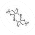
Embedded

A small embedded homeomorphic copy of rabbit in the center of a Julia set ^[3]

Fat

The fat rabbit or chubby rabbit has c at the root of the 1/3-limb of the Mandelbrot set. It has a parabolic fixed point with 3 petals. ^[4]

• 
  fat rabbit
• 
  parabolic chessboard

n-th eared

In general, the rabbit for the ${\displaystyle period-(n+1)}$th bulb of the main cardioid will have ${\displaystyle n}$ ears ^[5] For example, a period four bulb rabbit has three ears.

Perturbed

Perturbed rabbit ^[6]

• Perturbed rabbit
• 
  Perturbed rabbit
• 
  Perturbed rabbit zoom

Twisted rabbit problem

In the early 1980s, Hubbard posed the so-called twisted rabbit problem, a polynomial classification problem. The goal is to determine Thurston equivalence types^{[ definition needed ]} of functions of complex numbers that usually are not given by a formula (these are called topological polynomials): ^[7]

• given a topological quadratic whose branch point is periodic with period three, determining which quadratic polynomial it is Thurston equivalent to
• determining the equivalence class of twisted rabbits, i.e. composite of the rabbit polynomial with nth powers of Dehn twists about its ears.

The problem was originally solved by Laurent Bartholdi and Volodymyr Nekrashevych ^[8] using iterated monodromic groups. The generalization of the problem to the case where the number of post-critical points is arbitrarily large has been solved as well. ^[9]

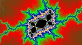
Gallery

• 
  Gray levels indicate the speed of convergence to infinity or to the attractive cycle
• 
  boundaries of level sets
• 
  binary decomposition
• 
• 
  with spine
• 
  with external rays
• 
  Multibrot-4 Douady rabbit
• 
  A Douady rabbit on a red background
• 
  A chain of Douady rabbits

See also

• Dragon curve
• Herman ring
• Siegel disc

References

1. "A Geometric Solution to the Twisted Rabbit Problem by Jim Belk, University of St Andrews" (PDF). Archived (PDF) from the original on 2022-11-01. Retrieved 2022-05-03.
2. Laurent Bartholdi; Volodymyr Nekrashevych (2006). "Thurston equivalence of topological polynomials". Acta Mathematica. 197: 1–51. arXiv: math/0510082 . doi:10.1007/s11511-006-0007-3.
3. "Period-n Rabbit Renormalization. 'Rabbit's show' by Evgeny Demidov". Archived from the original on 2022-05-03. Retrieved 2022-05-03.
4. Note on dynamically stable perturbations of parabolics by Tomoki Kawahira Archived October 2, 2006, at the Wayback Machine
5. "Twisted Three-Eared Rabbits: Identifying Topological Quadratics Up To Thurston Equivalence by Adam Chodof" (PDF). Archived (PDF) from the original on 2022-05-03. Retrieved 2022-05-03.
6. "Recent Research Papers (Only since 1999) Robert L. Devaney: Rabbits, Basilicas, and Other Julia Sets Wrapped in Sierpinski Carpets". Archived from the original on 2019-10-23. Retrieved 2020-04-07.
7. "Polynomials, dynamics, and trees by Becca Winarski" (PDF). Archived (PDF) from the original on 2022-11-01. Retrieved 2022-05-08.
8. Laurent Bartholdi; Volodymyr Nekrashevych (2005). "Thurston equivalence of topological polynomials". arXiv: math/0510082v3 .
9. James Belk; Justin Lanier; Dan Margalit; Rebecca R. Winarski (2019). "Recognizing Topological Polynomials by Lifting Trees". arXiv: 1906.07680v1 [math.DS].

External links

• Weisstein, Eric W. "Douady Rabbit Fractal". MathWorld .
• Dragt, A. "Lie Methods for Nonlinear Dynamics with Applications to Accelerator Physics".
• Adrien Douady: La dynamique du lapin (1996) - video on the YouTube

This article incorporates material from Douady Rabbit on PlanetMath, which is licensed under the Creative Commons Attribution/Share-Alike License.