List of fractals by Hausdorff dimension

According to Benoit Mandelbrot, "A fractal is by definition a set for which the Hausdorff-Besicovitch dimension strictly exceeds the topological dimension." ^[1] Presented here is a list of fractals, ordered by increasing Hausdorff dimension, to illustrate what it means for a fractal to have a low or a high dimension.

Deterministic fractals

Hausdorff dimension (exact value)	Hausdorff dimension (approx.)	Name	Illustration	Remarks
Calculated	0.538	Feigenbaum attractor		The Feigenbaum attractor (see between arrows) is the set of points generated by successive iterations of the logistic map for the critical parameter value ${\displaystyle \lambda _{\infty }=3.570}$, where the period doubling is infinite. This dimension is the same for any differentiable and unimodal function. [2]
${\displaystyle \log _{3}2}$	0.6309	Cantor set		Built by removing the central third at each iteration. Nowhere dense and not a countable set.
${\displaystyle {\frac {-\log 2}{\log \left(\displaystyle {\frac {1-\gamma }{2}}\right)}}}$	0<D<1	1D generalized symmetric Cantor set		Built by removing the central interval of length ${\displaystyle \gamma \,l_{n-1}}$ from each remaining interval of length ${\displaystyle l_{n-1}=(1-\gamma )^{n-1}/2^{n-1}}$ at the nth iteration. ${\displaystyle \gamma =1/3}$ produces the usual middle-third Cantor set. Varying ${\displaystyle \gamma }$ between 0 and 1 yields any fractal dimension ${\displaystyle 0<D<1}$. [3]
${\displaystyle \log _{2}\varphi =\log _{2}(1+{\sqrt {5}})-1}$	0.6942	(1/4, 1/2) asymmetric Cantor set		Built by removing the second quarter at each iteration. [4] ${\displaystyle \varphi =(1+{\sqrt {5}})/2}$ (golden ratio).
${\displaystyle \log _{10}5=1-\log _{10}2}$	0.69897	Real numbers whose base 10 digits are even		Similar to the Cantor set. [5]
${\displaystyle \log(1+{\sqrt {2}})}$	0.88137	Spectrum of Fibonacci Hamiltonian		The study of the spectrum of the Fibonacci Hamiltonian proves upper and lower bounds for its fractal dimension in the large coupling regime. These bounds show that the spectrum converges to an explicit constant. [6] [ page needed ]
${\displaystyle 1}$	1	Smith–Volterra–Cantor set		Built by removing the central interval of length ${\displaystyle 2^{-2n}}$ from each remaining interval at the nth iteration. Nowhere dense but has a Lebesgue measure of 1/2.
${\displaystyle 2+\log _{2}{\frac {1}{2}}=1}$	1	Takagi or Blancmange curve		Defined on the unit interval by ${\displaystyle f(x)=\sum \nolimits _{n=0}^{\infty }2^{-n}s(2^{n}x)}$, where ${\displaystyle s(x)}$ is the triangle wave function. Not a fractal under Mandelbrot's definition, because its topological dimension is also ${\displaystyle 1}$. [7] Special case of the Takahi-Landsberg curve: ${\displaystyle f(x)=\sum \nolimits _{n=0}^{\infty }w^{n}s(2^{n}x)}$ with ${\displaystyle w=1/2}$. The Hausdorff dimension equals ${\displaystyle 2+\log _{2}w}$ for ${\displaystyle w}$ in ${\displaystyle \left[1/2,1\right]}$. (Hunt cited by Mandelbrot [8] ).
Calculated	1.0812	Julia set z2 + 1/4		Julia set of f(z) = z2 + 1/4. [9]
Solution ${\displaystyle s}$ of ${\displaystyle 2|\alpha |^{3s}+|\alpha |^{4s}=1}$	1.0933	Boundary of the Rauzy fractal		Fractal representation introduced by G.Rauzy of the dynamics associated to the Tribonacci morphism: ${\displaystyle 1\mapsto 12}$, ${\displaystyle 2\mapsto 13}$ and ${\displaystyle 3\mapsto 1}$. [10] [ page needed ] [11] ${\displaystyle \alpha }$ is one of the conjugated roots of ${\displaystyle z^{3}-z^{2}-z-1=0}$.
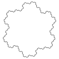
${\displaystyle 2\log _{7}3}$	1.12915	contour of the Gosper island		Term used by Mandelbrot (1977). [12] The Gosper island is the limit of the Gosper curve.
Measured (box counting)	1.2	Dendrite Julia set		Julia set of f(z) = z2 + i.
${\displaystyle {\frac {3\log \varphi }{\log \left(\displaystyle {\frac {3+{\sqrt {13}}}{2}}\right)}}}$	1.2083	Fibonacci word fractal 60°		Build from the Fibonacci word. See also the standard Fibonacci word fractal. ${\displaystyle \varphi =(1+{\sqrt {5}})/2}$ (golden ratio).
${\displaystyle {\begin{aligned}&2\log _{2}\left(\displaystyle {\frac {{\sqrt[{3}]{27-3{\sqrt {78}}}}+{\sqrt[{3}]{27+3{\sqrt {78}}}}}{3}}\right),\\&{\text{or root of }}2^{x}-1=2^{(2-x)/2}\end{aligned}}}$	1.2108	Boundary of the tame twindragon		One of the six 2-rep-tiles in the plane (can be tiled by two copies of itself, of equal size). [13] [14]
	1.26	Hénon map		The canonical Hénon map (with parameters a = 1.4 and b = 0.3) has Hausdorff dimension 1.261 ± 0.003. Different parameters yield different dimension values.
${\displaystyle \log _{3}4}$	1.2619	Triflake		Three anti-snowflakes arranged in a way that a koch-snowflake forms in between the anti-snowflakes.
${\displaystyle \log _{3}4}$	1.2619	Koch curve		3 Koch curves form the Koch snowflake or the anti-snowflake.
${\displaystyle \log _{3}4}$	1.2619	boundary of Terdragon curve		L-system: same as dragon curve with angle = 30°. The Fudgeflake is based on 3 initial segments placed in a triangle.
${\displaystyle \log _{3}4}$	1.2619	2D Cantor dust		Cantor set in 2 dimensions.
${\displaystyle \log _{3}4}$	1.2619	2D L-system branch		L-Systems branching pattern having 4 new pieces scaled by 1/3. Generating the pattern using statistical instead of exact self-similarity yields the same fractal dimension.
Calculated	1.2683	Julia set z2 − 1		Julia set of f(z) = z2 − 1. [9]
	1.3057	Apollonian gasket		Starting with 3 tangent circles, repeatedly packing new circles into the complementary interstices. Also the limit set generated by reflections in 4 mutually tangent circles. See [9]
	1.328	5 circles inversion fractal		The limit set generated by iterated inversions with respect to 5 mutually tangent circles (in red). Also an Apollonian packing. See [15]
${\displaystyle \log _{5}9}$	1.36521 [16]	Quadratic von Koch island using the type 1 curve as generator		Also known as the Minkowski Sausage
Calculated	1.3934	Douady rabbit		Julia set of f(z) = -0.123 + 0.745i [9]
${\displaystyle \log _{3}5}$	1.4649	Vicsek fractal		Built by exchanging iteratively each square by a cross of 5 squares.
${\displaystyle \log _{3}5}$	1.4649	Quadratic von Koch curve (type 1)		One can recognize the pattern of the Vicsek fractal (above).
${\displaystyle \log _{\sqrt {5}}{\frac {10}{3}}}$	1.4961	Quadric cross		The quadric cross is made by scaling the 3-segment generator unit by 5 then adding 3 full scaled units, one to each original segment, plus a third of a scaled unit (blue) to increase the length of the pedestal of the starting 3-segment unit (purple). Built by replacing each end segment with a cross segment scaled by a factor of 51/2, consisting of 3 1/3 new segments, as illustrated in the inset. Images generated with Fractal Generator for ImageJ.
${\displaystyle 2-\log _{2}{\sqrt {2}}={\frac {3}{2}}}$	1.5000	a Weierstrass function: ${\displaystyle f(x)=\sum _{k=1}^{\infty }{\frac {\sin(2^{k}x)}{{\sqrt {2}}^{\,k}}}}$		The Hausdorff dimension of the graph of the Weierstrass function ${\displaystyle f:[0,1]\to \mathbb {R} }$ defined by ${\displaystyle f(x)=\sum \nolimits _{k=1}^{\infty }a^{k}\sin(b^{k}x)}$ with ${\displaystyle 1/b<a<1}$ and ${\displaystyle b>1}$ is ${\displaystyle 2+\log _{b}a}$. [17] [18]
${\displaystyle \log _{4}8={\frac {3}{2}}}$	1.5000	Quadratic von Koch curve (type 2)		Also called "Minkowski sausage".
${\displaystyle \log _{2}\left({\frac {1+{\sqrt[{3}]{73-6{\sqrt {87}}}}+{\sqrt[{3}]{73+6{\sqrt {87}}}}}{3}}\right)}$	1.5236	Boundary of the Dragon curve		cf. Chang & Zhang. [19] [14]
${\displaystyle \log _{2}\left({\frac {1+{\sqrt[{3}]{73-6{\sqrt {87}}}}+{\sqrt[{3}]{73+6{\sqrt {87}}}}}{3}}\right)}$	1.5236	Boundary of the twindragon curve		Can be built with two dragon curves. One of the six 2-rep-tiles in the plane (can be tiled by two copies of itself, of equal size). [13]
${\displaystyle \log _{2}3}$	1.5850	3-branches tree		Each branch carries 3 branches (here 90° and 60°). The fractal dimension of the entire tree is the fractal dimension of the terminal branches. NB: the 2-branches tree has a fractal dimension of only 1.
${\displaystyle \log _{2}3}$	1.5850	Sierpinski triangle		Also the limiting shape of Pascal's triangle modulo 2.
${\displaystyle \log _{2}3}$	1.5850	Sierpiński arrowhead curve		Same limit as the triangle (above) but built with a one-dimensional curve.
${\displaystyle \log _{2}3}$	1.5850	Boundary of the T-square fractal		The dimension of the fractal itself (not the boundary) is ${\displaystyle \log _{2}4=2}$
${\displaystyle \log _{\sqrt[{\varphi }]{\varphi }}(\varphi )=\varphi }$	1.61803	a golden dragon		Built from two similarities of ratios ${\displaystyle r}$ and ${\displaystyle r^{2}}$, with ${\displaystyle r=1/\varphi ^{1/\varphi }}$. Its dimension equals ${\displaystyle \varphi }$ because ${\displaystyle ({r^{2}})^{\varphi }+r^{\varphi }=1}$. ${\displaystyle \varphi =(1+{\sqrt {5}})/2}$ (golden ratio).
${\displaystyle 1+\log _{3}2}$	1.6309	Pascal triangle modulo 3		For a triangle modulo k, if k is prime, the fractal dimension is ${\displaystyle 1+\log _{k}\left({\frac {k+1}{2}}\right)}$ (cf. Stephen Wolfram [20] ).
${\displaystyle 1+\log _{3}2}$	1.6309	Sierpinski Hexagon		Built in the manner of the Sierpinski carpet, on an hexagonal grid, with 6 similitudes of ratio 1/3. The Koch snowflake is present at all scales.
${\displaystyle {\frac {3\log \varphi }{\log(1+{\sqrt {2}})}}}$	1.6379	Fibonacci word fractal		Fractal based on the Fibonacci word (or Rabbit sequence) Sloane A005614. Illustration : Fractal curve after 23 steps (F23 = 28657 segments). [21] ${\displaystyle \varphi =(1+{\sqrt {5}})/2}$ (golden ratio).
Solution of ${\displaystyle (1/3)^{s}+(1/2)^{s}+(2/3)^{s}=1}$	1.6402	Attractor of IFS with 3 similarities of ratios 1/3, 1/2 and 2/3		Generalization : Providing the open set condition holds, the attractor of an iterated function system consisting of ${\displaystyle n}$ similarities of ratios ${\displaystyle c_{n}}$, has Hausdorff dimension ${\displaystyle s}$, solution of the equation coinciding with the iteration function of the Euclidean contraction factor: ${\displaystyle \sum \nolimits _{k=1}^{n}c_{k}^{s}=1}$. [5]
${\displaystyle \log _{8}32={\frac {5}{3}}}$	1.6667	32-segment quadric fractal (1/8 scaling rule)	see also: File:32 Segment One Eighth Scale Quadric Fractal.jpg	Generator for 32 segment 1/8 scale quadric fractal. Built by scaling the 32 segment generator (see inset) by 1/8 for each iteration, and replacing each segment of the previous structure with a scaled copy of the entire generator. The structure shown is made of 4 generator units and is iterated 3 times. The fractal dimension for the theoretical structure is log 32/log 8 = 1.6667. Images generated with Fractal Generator for ImageJ.
${\displaystyle 1+\log _{5}3}$	1.6826	Pascal triangle modulo 5		For a triangle modulo k, if k is prime, the fractal dimension is ${\displaystyle 1+\log _{k}\left({\frac {k+1}{2}}\right)}$ (cf. Stephen Wolfram [20] ).
Measured (box-counting)	1.7	Ikeda map attractor		For parameters a=1, b=0.9, k=0.4 and p=6 in the Ikeda map ${\displaystyle z_{n+1}=a+bz_{n}\exp \left[i\left[k-p/\left(1+\lfloor z_{n}\rfloor ^{2}\right)\right]\right]}$. It derives from a model of the plane-wave interactivity field in an optical ring laser. Different parameters yield different values. [22]
${\displaystyle 1+\log _{10}5}$	1.6990	50 segment quadric fractal (1/10 scaling rule)		Built by scaling the 50 segment generator (see inset) by 1/10 for each iteration, and replacing each segment of the previous structure with a scaled copy of the entire generator. The structure shown is made of 4 generator units and is iterated 3 times. The fractal dimension for the theoretical structure is log 50/log 10 = 1.6990. Images generated with Fractal Generator for ImageJ [23] . Generator for 50 Segment Fractal.
${\displaystyle 4\log _{5}2}$	1.7227	Pinwheel fractal		Built with Conway's Pinwheel tile.
${\displaystyle \log _{3}7}$	1.7712	Sphinx fractal		Built with the Sphinx hexiamond tiling, removing two of the nine sub-sphinxes. [24]
${\displaystyle \log _{3}7}$	1.7712	Hexaflake		Built by exchanging iteratively each hexagon by a flake of 7 hexagons. Its boundary is the von Koch flake and contains an infinity of Koch snowflakes (black or white).
${\displaystyle \log _{3}7}$	1.7712	Fractal H-I de Rivera		Starting from a unit square dividing its dimensions into three equal parts to form nine self-similar squares with the first square, two middle squares (the one that is above and the one below the central square) are removed in each of the seven squares not eliminated the process is repeated, so it continues indefinitely.
${\displaystyle {\frac {\log 4}{\log(2+2\cos(85^{\circ }))}}}$	1.7848	Von Koch curve 85°		Generalizing the von Koch curve with an angle a chosen between 0 and 90°. The fractal dimension is then ${\displaystyle {\frac {\log 4}{\log(2+2\cos a)}}\in [1,2]}$.
${\displaystyle \log _{2}\left(3^{0.63}+2^{0.63}\right)}$	1.8272	A self-affine fractal set		Build iteratively from a p-by-q array on a square, with ${\displaystyle p\leq q}$. Its Hausdorff dimension equals ${\displaystyle \log _{p}\left(\sum \nolimits _{k=1}^{p}n_{k}^{a}\right)}$ [5] with ${\displaystyle a=\log _{q}p}$ and ${\displaystyle n_{k}}$ is the number of elements in the ${\displaystyle k}$th column. The box-counting dimension yields a different formula, therefore, a different value. Unlike self-similar sets, the Hausdorff dimension of self-affine sets depends on the position of the iterated elements and there is no formula, so far, for the general case.
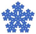
${\displaystyle {\frac {\log 6}{\log(1+\varphi )}}}$	1.8617	Pentaflake		Built by exchanging iteratively each pentagon by a flake of 6 pentagons. ${\displaystyle \varphi =(1+{\sqrt {5}})/2}$ (golden ratio).
solution of ${\displaystyle 6(1/3)^{s}+5{(1/3{\sqrt {3}})}^{s}=1}$	1.8687	Monkeys tree		This curve appeared in Benoit Mandelbrot's "Fractal geometry of Nature" (1983). It is based on 6 similarities of ratio ${\displaystyle 1/3}$ and 5 similarities of ratio ${\displaystyle 1/3{\sqrt {3}}}$. [25]
${\displaystyle \log _{3}8}$	1.8928	Sierpinski carpet		Each face of the Menger sponge is a Sierpinski carpet, as is the bottom surface of the 3D quadratic Koch surface (type 1).
${\displaystyle \log _{3}8}$	1.8928	3D Cantor dust		Cantor set in 3 dimensions.
${\displaystyle \log _{3}4+\log _{3}2={\frac {\log 4}{\log 3}}+{\frac {\log 2}{\log 3}}={\frac {\log 8}{\log 3}}}$	1.8928	Cartesian product of the von Koch curve and the Cantor set		Generalization : Let F×G be the cartesian product of two fractals sets F and G. Then ${\displaystyle \dim _{H}(F\times G)=\dim _{H}F+\dim _{H}G}$. [5] See also the 2D Cantor dust and the Cantor cube.
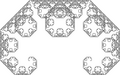
${\displaystyle 2\log _{2}x}$ where ${\displaystyle x^{9}-3x^{8}+3x^{7}-3x^{6}+2x^{5}+4x^{4}-8x^{3}+}$${\displaystyle 8x^{2}-16x+8=0}$	1.9340	Boundary of the Lévy C curve		Estimated by Duvall and Keesling (1999). The curve itself has a fractal dimension of 2.
	2	Penrose tiling		See Ramachandrarao, Sinha & Sanyal. [26]
${\displaystyle 2}$	2	Boundary of the Mandelbrot set		The boundary and the set itself have the same Hausdorff dimension. [27]
${\displaystyle 2}$	2	Julia set		For determined values of c (including c belonging to the boundary of the Mandelbrot set), the Julia set has a dimension of 2. [27]
${\displaystyle 2}$	2	Sierpiński curve		Every space-filling curve filling the plane has a Hausdorff dimension of 2.
${\displaystyle 2}$	2	Hilbert curve
${\displaystyle 2}$	2	Peano curve		And a family of curves built in a similar way, such as the Wunderlich curves.
${\displaystyle 2}$	2	Moore curve		Can be extended in 3 dimensions.
	2	Lebesgue curve or z-order curve		Unlike the previous ones this space-filling curve is differentiable almost everywhere. Another type can be defined in 2D. Like the Hilbert Curve it can be extended in 3D. [28]
${\displaystyle \log _{\sqrt {2}}2=2}$	2	Dragon curve		And its boundary has a fractal dimension of 1.5236270862. [29]
	2	Terdragon curve		L-system: F → F + F – F, angle = 120°.
${\displaystyle \log _{2}4=2}$	2	Gosper curve		Its boundary is the Gosper island.
Solution of ${\displaystyle 7({1/3})^{s}+6({1/3{\sqrt {3}}})^{s}=1}$	2	Curve filling the Koch snowflake		Proposed by Mandelbrot in 1982, [30] it fills the Koch snowflake. It is based on 7 similarities of ratio 1/3 and 6 similarities of ratio ${\displaystyle 1/3{\sqrt {3}}}$.
${\displaystyle \log _{2}4=2}$	2	Sierpiński tetrahedron		Each tetrahedron is replaced by 4 tetrahedra.
${\displaystyle \log _{2}4=2}$	2	H-fractal		Also the Mandelbrot tree which has a similar pattern.
${\displaystyle {\frac {\log 2}{\log(2/{\sqrt {2}})}}=2}$	2	Pythagoras tree (fractal)		Every square generates two squares with a reduction ratio of ${\displaystyle 1/{\sqrt {2}}}$.
${\displaystyle \log _{2}4=2}$	2	2D Greek cross fractal		Each segment is replaced by a cross formed by 4 segments.
Measured	2.01 ± 0.01	Rössler attractor		The fractal dimension of the Rössler attractor is slightly above 2. For a=0.1, b=0.1 and c=14 it has been estimated between 2.01 and 2.02. [31]
Measured	2.06 ± 0.01	Lorenz attractor		For parameters ${\displaystyle \rho =40}$, ${\displaystyle \sigma =16}$ and ${\displaystyle \beta =4}$ . See McGuinness (1983) [32]
${\displaystyle 4+c^{D}+d^{D}=(c+d)^{D}}$	2<D<2.3	Pyramid surface		Each triangle is replaced by 6 triangles, of which 4 identical triangles form a diamond based pyramid and the remaining two remain flat with lengths ${\displaystyle c}$ and ${\displaystyle d}$ relative to the pyramid triangles. The dimension is a parameter, self-intersection occurs for values greater than 2.3. [33]
${\displaystyle \log _{2}5}$	2.3219	Fractal pyramid		Each square pyramid is replaced by 5 half-size square pyramids. (Different from the Sierpinski tetrahedron, which replaces each triangular pyramid with 4 half-size triangular pyramids).
${\displaystyle {\frac {\log 20}{\log(2+\varphi )}}}$	2.3296	Dodecahedron fractal		Each dodecahedron is replaced by 20 dodecahedra. ${\displaystyle \varphi =(1+{\sqrt {5}})/2}$ (golden ratio).
${\displaystyle \log _{3}13}$	2.3347	3D quadratic Koch surface (type 1)		Extension in 3D of the quadratic Koch curve (type 1). The illustration shows the first (blue block), second (plus green blocks), third (plus yellow blocks) and fourth (plus clear blocks) iterations.
	2.4739	Apollonian sphere packing		The interstice left by the Apollonian spheres. Apollonian gasket in 3D. Dimension calculated by M. Borkovec, W. De Paris, and R. Peikert. [34]
${\displaystyle \log _{4}32={\frac {5}{2}}}$	2.50	3D quadratic Koch surface (type 2)		Extension in 3D of the quadratic Koch curve (type 2). The illustration shows the second iteration.
${\displaystyle {\frac {\log \left({\frac {\sqrt {7}}{6}}-{\frac {1}{3}}\right)}{\log({\sqrt {2}}-1)}}}$	2.529	Jerusalem cube		The iteration n is built with 8 cubes of iteration n−1 (at the corners) and 12 cubes of iteration n-2 (linking the corners). The contraction ratio is ${\displaystyle {\sqrt {2}}-1}$.
${\displaystyle {\frac {\log 12}{\log(1+\varphi )}}}$	2.5819	Icosahedron fractal		Each icosahedron is replaced by 12 icosahedra. ${\displaystyle \varphi =(1+{\sqrt {5}})/2}$ (golden ratio).
${\displaystyle 1+\log _{2}3}$	2.5849	3D Greek cross fractal		Each segment is replaced by a cross formed by 6 segments.
${\displaystyle 1+\log _{2}3}$	2.5849	Octahedron fractal		Each octahedron is replaced by 6 octahedra.
${\displaystyle 1+\log _{2}3}$	2.5849	von Koch surface		Each equilateral triangular face is cut into 4 equal triangles. Using the central triangle as the base, form a tetrahedron. Replace the triangular base with the tetrahedral "tent".
${\displaystyle {\frac {\log 3}{\log(3/2)}}}$	2.7095	Von Koch in 3D		Start with a 6-sided polyhedron whose faces are isosceles triangles with sides of ratio 2:2:3 . Replace each polyhedron with 3 copies of itself, 2/3 smaller. [35]
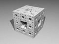
${\displaystyle \log _{3}20}$	2.7268	Menger sponge		And its surface has a fractal dimension of ${\displaystyle \log _{3}20}$, which is the same as that by volume.
${\displaystyle \log _{2}8=3}$	3	3D Hilbert curve		A Hilbert curve extended to 3 dimensions.
${\displaystyle \log _{2}8=3}$	3	3D Lebesgue curve		A Lebesgue curve extended to 3 dimensions.
${\displaystyle \log _{2}8=3}$	3	3D Moore curve		A Moore curve extended to 3 dimensions.
${\displaystyle \log _{2}8=3}$	3	3D H-fractal		A H-fractal extended to 3 dimensions. [36]
${\displaystyle 3}$ (conjectured)	3 (to be confirmed)	Mandelbulb		Extension of the Mandelbrot set (power 9) in 3 dimensions [37] [ unreliable source? ]

Random and natural fractals

Hausdorff dimension (exact value)	Hausdorff dimension (approx.)	Name	Illustration	Remarks
${\displaystyle {\frac {1}{2}}}$	0.5	Zeros of a Wiener process		The zeros of a Wiener process (Brownian motion) are a nowhere dense set of Lebesgue measure 0 with a fractal structure. [5] [38]
Solution of ${\displaystyle E(C_{1}^{s}+C_{2}^{s})=1}$ where ${\displaystyle E(C_{1})=0.5}$ and ${\displaystyle E(C_{2})=0.3}$	0.7499	a random Cantor set with 50% - 30%		Generalization: at each iteration, the length of the left interval is defined with a random variable ${\displaystyle C_{1}}$, a variable percentage of the length of the original interval. Same for the right interval, with a random variable ${\displaystyle C_{2}}$. Its Hausdorff Dimension ${\displaystyle s}$ satisfies: ${\displaystyle E(C_{1}^{s}+C_{2}^{s})=1}$ (where ${\displaystyle E(X)}$ is the expected value of ${\displaystyle X}$). [5]
Solution of ${\displaystyle s+1=12\cdot 2^{-(s+1)}-6\cdot 3^{-(s+1)}}$	1.144...	von Koch curve with random interval		The length of the middle interval is a random variable with uniform distribution on the interval (0,1/3). [5]
Measured	1.22 ± 0.02	Coastline of Ireland		Values for the fractal dimension of the entire coast of Ireland were determined by McCartney, Abernethy and Gault [39] at the University of Ulster and Theoretical Physics students at Trinity College, Dublin, under the supervision of S. Hutzler. [40] Note that there are marked differences between Ireland's ragged west coast (fractal dimension of about 1.26) and the much smoother east coast (fractal dimension 1.10) [40]
Measured	1.25	Coastline of Great Britain		Fractal dimension of the west coast of Great Britain, as measured by Lewis Fry Richardson and cited by Benoît Mandelbrot. [41]
${\displaystyle {\frac {\log 4}{\log 3}}}$	1.2619	von Koch curve with random orientation		One introduces here an element of randomness which does not affect the dimension, by choosing, at each iteration, to place the equilateral triangle above or below the curve. [5]
${\displaystyle {\frac {4}{3}}}$	1.333	Boundary of Brownian motion		(cf. Mandelbrot, Lawler, Schramm, Werner). [42]
${\displaystyle {\frac {4}{3}}}$	1.333	Polymer in 2D		Similar to the Brownian motion in 2D with non-self-intersection. [43]
${\displaystyle {\frac {4}{3}}}$	1.333	Percolation front in 2D, Corrosion front in 2D		Fractal dimension of the percolation-by-invasion front (accessible perimeter), at the percolation threshold (59.3%). It's also the fractal dimension of a stopped corrosion front. [43]
	1.40	Clusters of clusters 2D		When limited by diffusion, clusters combine progressively to a unique cluster of dimension 1.4. [43]
${\displaystyle 2-{\frac {1}{2}}}$	1.5	Graph of a regular Brownian function (Wiener process)		Graph of a function ${\displaystyle f}$ such that, for any two positive reals ${\displaystyle x}$ and ${\displaystyle x+h}$, the difference of their images ${\displaystyle f(x+h)-f(x)}$ has the centered gaussian distribution with variance ${\displaystyle h}$. Generalization: the fractional Brownian motion of index ${\displaystyle \alpha }$ follows the same definition but with a variance ${\displaystyle h^{2\alpha }}$, in that case its Hausdorff dimension equals ${\displaystyle 2-\alpha }$. [5]
Measured	1.52	Coastline of Norway		See J. Feder. [44]
Measured	1.55	Self-avoiding walk		Random walk in a square lattice that avoids visiting the same place twice, with a "go-back" routine for avoiding dead ends.
${\displaystyle {\frac {5}{3}}}$	1.66	Polymer in 3D		Similar to the Brownian motion in a cubic lattice, but without self-intersection. [43]
	1.70	2D DLA Cluster		In 2 dimensions, clusters formed by diffusion-limited aggregation, have a fractal dimension of around 1.70. [43]
${\displaystyle {\frac {\log(9\cdot 0.75)}{\log 3}}}$	1.7381	Fractal percolation with 75% probability		The fractal percolation model is constructed by the progressive replacement of each square by a 3-by-3 grid in which is placed a random collection of sub-squares, each sub-square being retained with probability p. The "almost sure" Hausdorff dimension equals ${\displaystyle {\frac {\log(9p)}{\log 3}}}$. [5]
${\displaystyle {\frac {7}{4}}}$	1.75	2D percolation cluster hull		The hull or boundary of a percolation cluster. Can also be generated by a hull-generating walk, [45] or by Schramm-Loewner Evolution.
${\displaystyle {\frac {91}{48}}}$	1.8958	2D percolation cluster		In a square lattice, under the site percolation threshold (59.3%) the percolation-by-invasion cluster has a fractal dimension of 91/48. [43] [46] Beyond that threshold, the cluster is infinite and 91/48 becomes the fractal dimension of the "clearings".
${\displaystyle {\frac {\log 2}{\log {\sqrt {2}}}}=2}$	2	Brownian motion		Or random walk. The Hausdorff dimensions equals 2 in 2D, in 3D and in all greater dimensions (K.Falconer "The geometry of fractal sets").
Measured	Around 2	Distribution of galaxy clusters		From the 2005 results of the Sloan Digital Sky Survey. [47]
	2.5	Balls of crumpled paper		When crumpling sheets of different sizes but made of the same type of paper and with the same aspect ratio (for example, different sizes in the ISO 216 A series), then the diameter of the balls so obtained elevated to a non-integer exponent between 2 and 3 will be approximately proportional to the area of the sheets from which the balls have been made. [48] Creases will form at all size scales (see Universality (dynamical systems)).
	2.50	3D DLA Cluster		In 3 dimensions, clusters formed by diffusion-limited aggregation, have a fractal dimension of around 2.50. [43]
	2.50	Lichtenberg figure		Their appearance and growth appear to be related to the process of diffusion-limited aggregation or DLA. [43]
${\displaystyle 3-{\frac {1}{2}}}$	2.5	regular Brownian surface		A function ${\displaystyle f:\mathbb {R} ^{2}\to \mathbb {R} }$, gives the height of a point ${\displaystyle (x,y)}$ such that, for two given positive increments ${\displaystyle h}$ and ${\displaystyle k}$, then ${\displaystyle f(x+h,y+k)-f(x,y)}$ has a centered Gaussian distribution with variance ${\displaystyle {\sqrt {h^{2}+k^{2}}}}$. Generalization: the fractional Brownian surface of index ${\displaystyle \alpha }$ follows the same definition but with a variance ${\displaystyle (h^{2}+k^{2})^{\alpha }}$, in that case its Hausdorff dimension equals ${\displaystyle 3-\alpha }$. [5]
Measured	2.52	3D percolation cluster		In a cubic lattice, at the site percolation threshold (31.1%), the 3D percolation-by-invasion cluster has a fractal dimension of around 2.52. [46] Beyond that threshold, the cluster is infinite.
Measured and calculated	~2.7	The surface of Broccoli		San-Hoon Kim used a direct scanning method and a cross section analysis of a broccoli to conclude that the fractal dimension of it is ~2.7. [49]
Measured	~2.8	Surface of human brain		Measured with segmented three-dimensional high-resolution magnetic resonance images [50]
Measured and calculated	~2.8	Cauliflower		San-Hoon Kim used a direct scanning method and a mathematical analysis of the cross section of a cauliflower to conclude that the fractal dimension of it is ~2.8. [49]
	2.97	Lung surface		The alveoli of a lung form a fractal surface close to 3. [43]
Calculated	${\displaystyle \in (0,2)}$	Multiplicative cascade		This is an example of a multifractal distribution. However, by choosing its parameters in a particular way we can force the distribution to become a monofractal. [51]

See also

• Fractal dimension
• Hausdorff dimension
• Scale invariance

Notes and references

1. Mandelbrot 1982 , p. 15
2. Aurell, Erik (May 1987). "On the metric properties of the Feigenbaum attractor". Journal of Statistical Physics. 47 (3–4): 439–458. Bibcode:1987JSP....47..439A. doi:10.1007/BF01007519. S2CID   122213380.
3. Cherny, A. Yu; Anitas, E.M.; Kuklin, A.I.; Balasoiu, M.; Osipov, V.A. (2010). "The scattering from generalized Cantor fractals". J. Appl. Crystallogr. 43 (4): 790–7. arXiv: 0911.2497 . doi:10.1107/S0021889810014184. S2CID   94779870.
4. Tsang, K. Y. (1986). "Dimensionality of Strange Attractors Determined Analytically". Phys. Rev. Lett. 57 (12): 1390–1393. Bibcode:1986PhRvL..57.1390T. doi:10.1103/PhysRevLett.57.1390. PMID   10033437.
5. Falconer, Kenneth (1990–2003). Fractal Geometry: Mathematical Foundations and Applications. John Wiley & Sons, Ltd. xxv. ISBN   978-0-470-84862-3.
6. Damanik, D.; Embree, M.; Gorodetski, A.; Tcheremchantse, S. (2008). "The Fractal Dimension of the Spectrum of the Fibonacci Hamiltonian". Commun. Math. Phys. 280 (2): 499–516. arXiv: 0705.0338 . Bibcode:2008CMaPh.280..499D. doi:10.1007/s00220-008-0451-3. S2CID   12245755.
7. Vaz, Cristina (2019). Noções Elementares Sobre Dimensão. ISBN   9788565054867.
8. Mandelbrot, Benoit (2002). Gaussian self-affinity and Fractals. Springer. ISBN   978-0-387-98993-8.
9. McMullen, Curtis T. (3 October 1997). "Hausdorff dimension and conformal dynamics III: Computation of dimension", Abel.Math.Harvard.edu. Accessed: 27 October 2018.
10. Messaoudi, Ali. Frontième de numération complexe", matwbn.icm.edu.pl. (in French) Accessed: 27 October 2018.
11. Lothaire, M. (2005), Applied combinatorics on words, Encyclopedia of Mathematics and its Applications, vol. 105, Cambridge University Press, p.  525, ISBN   978-0-521-84802-2, MR   2165687, Zbl   1133.68067
12. Weisstein, Eric W. "Gosper Island". MathWorld . Retrieved 27 October 2018.
13. Ngai, Sirvent, Veerman, and Wang (October 2000). "On 2-Reptiles in the Plane 1999", Geometriae Dedicata, Volume 82. Accessed: 29 October 2018.
14. Duda, Jarek (March 2011). "The Boundary of Periodic Iterated Function Systems", Wolfram.com.
15. Chang, Angel and Zhang, Tianrong. "On the Fractal Structure of the Boundary of Dragon Curve". Archived from the original on 14 June 2011. Retrieved 9 February 2019. pdf
16. Mandelbrot, B. B. (1983). The Fractal Geometry of Nature, p.48. New York: W. H. Freeman. ISBN   9780716711865. Cited in: Weisstein, Eric W. "Minkowski Sausage". MathWorld . Retrieved 22 September 2019.
17. Shen, Weixiao (2018). "Hausdorff dimension of the graphs of the classical Weierstrass functions". Mathematische Zeitschrift. 289 (1–2): 223–266. arXiv: 1505.03986 . doi:10.1007/s00209-017-1949-1. ISSN   0025-5874. S2CID   118844077.
18. N. Zhang. The Hausdorff dimension of the graphs of fractal functions. (In Chinese). Master Thesis. Zhejiang University, 2018.
19. Fractal dimension of the boundary of the dragon fractal
20. "Fractal dimension of the Pascal triangle modulo k". Archived from the original on 15 October 2012. Retrieved 2 October 2006.
21. The Fibonacci word fractal
22. Theiler, James (1990). "Estimating fractal dimension" (PDF). J. Opt. Soc. Am. A. 7 (6): 1055–73. Bibcode:1990JOSAA...7.1055T. doi:10.1364/JOSAA.7.001055.
23. Fractal Generator for ImageJ Archived 20 March 2012 at the Wayback Machine .
24. W. Trump, G. Huber, C. Knecht, R. Ziff, to be published
25. Monkeys tree fractal curve Archived 21 September 2002 at archive.today
26. Fractal dimension of a Penrose tiling
27. Shishikura, Mitsuhiro (1991). "The Hausdorff dimension of the boundary of the Mandelbrot set and Julia sets". arXiv: math/9201282 .
28. Lebesgue curve variants
29. Duda, Jarek (2008). "Complex base numeral systems". arXiv: 0712.1309v3 [math.DS].
30. Seuil (1982). Penser les mathématiques. Seuil. ISBN   2-02-006061-2.
31. Fractals and the Rössler attractor
32. McGuinness, M.J. (1983). "The fractal dimension of the Lorenz attractor". Physics Letters. 99A (1): 5–9. Bibcode:1983PhLA...99....5M. doi:10.1016/0375-9601(83)90052-X.
33. Lowe, Thomas (24 October 2016). "Three Variable Dimension Surfaces". ResearchGate.
34. The Fractal dimension of the apollonian sphere packing Archived 6 May 2016 at the Wayback Machine
35. Baird, Eric (2014). "The Koch curve in three dimensions" – via ResearchGate.
36. Hou, B.; Xie, H.; Wen, W.; Sheng, P. (2008). "Three-dimensional metallic fractals and their photonic crystal characteristics" (PDF). Phys. Rev. B. 77 (12): 125113. Bibcode:2008PhRvB..77l5113H. doi:10.1103/PhysRevB.77.125113.
37. Hausdorff dimension of the Mandelbulb
38. Peter Mörters, Yuval Peres, "Brownian Motion", Cambridge University Press, 2010
39. McCartney, Mark; Abernethya, Gavin; Gaulta, Lisa (24 June 2010). "The Divider Dimension of the Irish Coast". Irish Geography. 43 (3): 277–284. doi:10.1080/00750778.2011.582632.
40. Hutzler, S. (2013). "Fractal Ireland". Science Spin. 58: 19–20. Retrieved 15 November 2016. (See contents page, archived 26 July 2013)
41. How long is the coast of Britain? Statistical self-similarity and fractional dimension, B. Mandelbrot
42. Lawler, Gregory F.; Schramm, Oded; Werner, Wendelin (2001). "The Dimension of the Planar Brownian Frontier is 4/3". Math. Res. Lett. 8 (4): 401–411. arXiv: math/0010165 . Bibcode:2000math.....10165L. doi:10.4310/MRL.2001.v8.n4.a1. S2CID   5877745.
43. Sapoval, Bernard (2001). Universalités et fractales. Flammarion-Champs. ISBN   2-08-081466-4.
44. Feder, J., "Fractals", Plenum Press, New York, (1988).
45. Hull-generating walks
46. M Sahini; M Sahimi (2003). Applications Of Percolation Theory. CRC Press. ISBN   978-0-203-22153-2.
47. Basic properties of galaxy clustering in the light of recent results from the Sloan Digital Sky Survey
48. "Power Law Relations". Yale. Archived from the original on 28 June 2010. Retrieved 29 July 2010.{{cite journal}}: Cite journal requires |journal= (help)
49. Kim, Sang-Hoon (2 February 2008). "Fractal dimensions of a green broccoli and a white cauliflower". arXiv: cond-mat/0411597 .
50. Kiselev, Valerij G.; Hahn, Klaus R.; Auer, Dorothee P. (2003). "Is the brain cortex a fractal?". NeuroImage. 20 (3): 1765–1774. doi:10.1016/S1053-8119(03)00380-X. PMID   14642486. S2CID   14240006.
51. Meakin, Paul (1987). "Diffusion-limited aggregation on multifractal lattices: A model for fluid-fluid displacement in porous media". Physical Review A. 36 (6): 2833–2837. Bibcode:1987PhRvA..36.2833M. doi:10.1103/PhysRevA.36.2833. PMID   9899187.

Further reading

• Mandelbrot, Benoît (1982). The Fractal Geometry of Nature . W.H. Freeman. ISBN   0-7167-1186-9.
• Peitgen, Heinz-Otto (1988). Saupe, Dietmar (ed.). The Science of Fractal Images . Springer Verlag. ISBN   0-387-96608-0.
• Barnsley, Michael F. (1 January 1993). Fractals Everywhere. Morgan Kaufmann. ISBN   0-12-079061-0.
• Sapoval, Bernard; Mandelbrot, Benoît B. (2001). Universalités et fractales: jeux d'enfant ou délits d'initié?. Flammarion-Champs. ISBN   2-08-081466-4.

External links

• The fractals on Mathworld
• Other fractals on Paul Bourke's website
• Soler's Gallery
• Fractals on mathcurve.com
• 1000fractales.free.fr - Project gathering fractals created with various software
• Fractals unleashed
• IFStile - software that computes the dimension of the boundary of self-affine tiles