Discrete wavelet transform

An example of the 2D discrete wavelet transform that is used in JPEG2000. The original image is high-pass filtered, yielding the three large images, each describing local changes in brightness (details) in the original image. It is then low-pass filtered and downscaled, yielding an approximation image; this image is high-pass filtered to produce the three smaller detail images, and low-pass filtered to produce the final approximation image in the upper-left.

In numerical analysis and functional analysis, a discrete wavelet transform (DWT) is any wavelet transform for which the wavelets are discretely sampled. As with other wavelet transforms, a key advantage it has over Fourier transforms is temporal resolution: it captures both frequency and location information (location in time).

Definition

One level of the transform

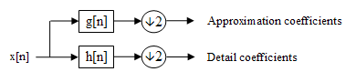
The DWT of a signal ${\displaystyle x}$ is calculated by passing it through a series of filters. First the samples are passed through a low-pass filter with impulse response ${\displaystyle g}$ resulting in a convolution of the two:

${\displaystyle y[n]=(x*g)[n]=\sum \limits _{k=-\infty }^{\infty }{x[k]g[n-k]}}$

The signal is also decomposed simultaneously using a high-pass filter ${\displaystyle h}$. The outputs give the detail coefficients (from the high-pass filter) and approximation coefficients (from the low-pass). It is important that the two filters are related to each other and they are known as a quadrature mirror filter.

Block diagram of filter analysis

However, since half the frequencies of the signal have now been removed, half the samples can be discarded according to Nyquist's rule. The filter output of the low-pass filter ${\displaystyle g}$ in the diagram above is then subsampled by 2 and further processed by passing it again through a new low-pass filter ${\displaystyle g}$ and a high- pass filter ${\displaystyle h}$ with half the cut-off frequency of the previous one, i.e.:

${\displaystyle y_{\mathrm {low} }[n]=\sum \limits _{k=-\infty }^{\infty }{x[k]g[2n-k]}}$

${\displaystyle y_{\mathrm {high} }[n]=\sum \limits _{k=-\infty }^{\infty }{x[k]h[2n-k]}}$

This decomposition has halved the time resolution since only half of each filter output characterises the signal. However, each output has half the frequency band of the input, so the frequency resolution has been doubled.

With the subsampling operator ${\displaystyle \downarrow }$

${\displaystyle (y\downarrow k)[n]=y[kn]}$

the above summation can be written more concisely.

${\displaystyle y_{\mathrm {low} }=(x*g)\downarrow 2}$

${\displaystyle y_{\mathrm {high} }=(x*h)\downarrow 2}$

However computing a complete convolution ${\displaystyle x*g}$ with subsequent downsampling would waste computation time.

The Lifting scheme is an optimization where these two computations are interleaved.

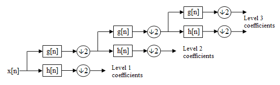
Cascading and filter banks

This decomposition is repeated to further increase the frequency resolution and the approximation coefficients decomposed with high- and low-pass filters and then down-sampled. This is represented as a binary tree with nodes representing a sub-space with a different time-frequency localisation. The tree is known as a filter bank.

A 3 level filter bank

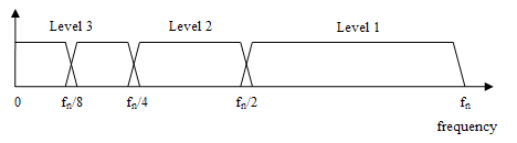
At each level in the above diagram the signal is decomposed into low and high frequencies. Due to the decomposition process the input signal must be a multiple of ${\displaystyle 2^{n}}$ where ${\displaystyle n}$ is the number of levels.

For example a signal with 32 samples, frequency range 0 to ${\displaystyle f_{n}}$ and 3 levels of decomposition, 4 output scales are produced:

Level	Frequencies	Samples
3	${\displaystyle 0}$ to ${\displaystyle {f_{n}}/8}$	4
	${\displaystyle {f_{n}}/8}$ to ${\displaystyle {f_{n}}/4}$	4
2	${\displaystyle {f_{n}}/4}$ to ${\displaystyle {f_{n}}/2}$	8
1	${\displaystyle {f_{n}}/2}$ to ${\displaystyle f_{n}}$	16

Frequency domain representation of the DWT

Relationship to the mother wavelet

The filterbank implementation of wavelets can be interpreted as computing the wavelet coefficients of a discrete set of child wavelets for a given mother wavelet ${\displaystyle \psi (t)}$. In the case of the discrete wavelet transform, the mother wavelet is shifted and scaled by powers of two

${\displaystyle \psi _{j,k}(t)={\frac {1}{\sqrt {2^{j}}}}\psi \left({\frac {t-k2^{j}}{2^{j}}}\right)}$

where ${\displaystyle j}$ is the scale parameter and ${\displaystyle k}$ is the shift parameter, both of which are integers.

Recall that the wavelet coefficient ${\displaystyle \gamma }$ of a signal ${\displaystyle x(t)}$ is the projection of ${\displaystyle x(t)}$ onto a wavelet, and let ${\displaystyle x(t)}$ be a signal of length ${\displaystyle 2^{N}}$. In the case of a child wavelet in the discrete family above,

${\displaystyle \gamma _{jk}=\int _{-\infty }^{\infty }x(t){\frac {1}{\sqrt {2^{j}}}}\psi \left({\frac {t-k2^{j}}{2^{j}}}\right)dt}$

Now fix ${\displaystyle j}$ at a particular scale, so that ${\displaystyle \gamma _{jk}}$ is a function of ${\displaystyle k}$ only. In light of the above equation, ${\displaystyle \gamma _{jk}}$ can be viewed as a convolution of ${\displaystyle x(t)}$ with a dilated, reflected, and normalized version of the mother wavelet, ${\displaystyle h(t)={\frac {1}{\sqrt {2^{j}}}}\psi \left({\frac {-t}{2^{j}}}\right)}$, sampled at the points ${\displaystyle 1,2^{j},2\cdot {2^{j}},...,2^{N}}$. But this is precisely what the detail coefficients give at level ${\displaystyle j}$ of the discrete wavelet transform. Therefore, for an appropriate choice of ${\displaystyle h[n]}$ and ${\displaystyle g[n]}$, the detail coefficients of the filter bank correspond exactly to a wavelet coefficient of a discrete set of child wavelets for a given mother wavelet ${\displaystyle \psi (t)}$.

As an example, consider the discrete Haar wavelet, whose mother wavelet is ${\displaystyle \psi =[1,-1]}$. Then the dilated, reflected, and normalized version of this wavelet is ${\displaystyle h[n]={\frac {1}{\sqrt {2}}}[-1,1]}$, which is, indeed, the highpass decomposition filter for the discrete Haar wavelet transform.

Time complexity

The filterbank implementation of the Discrete Wavelet Transform takes only O(N) in certain cases, as compared to O(N log N) for the fast Fourier transform.

Note that if ${\displaystyle g[n]}$ and ${\displaystyle h[n]}$ are both a constant length (i.e. their length is independent of N), then ${\displaystyle x*h}$ and ${\displaystyle x*g}$ each take O(N) time. The wavelet filterbank does each of these two O(N) convolutions, then splits the signal into two branches of size N/2. But it only recursively splits the upper branch convolved with ${\displaystyle g[n]}$ (as contrasted with the FFT, which recursively splits both the upper branch and the lower branch). This leads to the following recurrence relation

${\displaystyle T(N)=2N+T\left({\frac {N}{2}}\right)}$

which leads to an O(N) time for the entire operation, as can be shown by a geometric series expansion of the above relation.

As an example, the discrete Haar wavelet transform is linear, since in that case ${\displaystyle h[n]}$ and ${\displaystyle g[n]}$ are constant length 2.

${\displaystyle h[n]=\left[{\frac {-{\sqrt {2}}}{2}},{\frac {\sqrt {2}}{2}}\right]g[n]=\left[{\frac {\sqrt {2}}{2}},{\frac {\sqrt {2}}{2}}\right]}$

The locality of wavelets, coupled with the O(N) complexity, guarantees that the transform can be computed online (on a streaming basis). This property is in sharp contrast to FFT, which requires access to the entire signal at once. It also applies to the multi-scale transform and also to the multi-dimensional transforms (e.g., 2-D DWT). ^[1]

Examples

Haar wavelets

Main article: Haar wavelet

The first DWT was invented by Hungarian mathematician Alfréd Haar. For an input represented by a list of ${\displaystyle 2^{n}}$ numbers, the Haar wavelet transform may be considered to pair up input values, storing the difference and passing the sum. This process is repeated recursively, pairing up the sums to prove the next scale, which leads to ${\displaystyle 2^{n}-1}$ differences and a final sum.

Daubechies wavelets

Main article: Daubechies wavelet

The most commonly used set of discrete wavelet transforms was formulated by the Belgian mathematician Ingrid Daubechies in 1988. This formulation is based on the use of recurrence relations to generate progressively finer discrete samplings of an implicit mother wavelet function; each resolution is twice that of the previous scale. In her seminal paper, Daubechies derives a family of wavelets, the first of which is the Haar wavelet. Interest in this field has exploded since then, and many variations of Daubechies' original wavelets were developed. ^{[2] [3] [4]}

The dual-tree complex wavelet transform (DCWT)

Main article: Complex wavelet transform

The dual-tree complex wavelet transform (${\displaystyle \mathbb {C} }$WT) is a relatively recent enhancement to the discrete wavelet transform (DWT), with important additional properties: It is nearly shift invariant and directionally selective in two and higher dimensions. It achieves this with a redundancy factor of only ${\displaystyle 2^{d}}$, substantially lower than the undecimated DWT. The multidimensional (M-D) dual-tree ${\displaystyle \mathbb {C} }$WT is nonseparable but is based on a computationally efficient, separable filter bank (FB). ^[5]

Others

Other forms of discrete wavelet transform include the Le Gall–Tabatabai (LGT) 5/3 wavelet developed by Didier Le Gall and Ali J. Tabatabai in 1988 (used in JPEG 2000 or JPEG XS ), ^{[6] [7] [8]} the Binomial QMF developed by Ali Naci Akansu in 1990, ^[9] the set partitioning in hierarchical trees (SPIHT) algorithm developed by Amir Said with William A. Pearlman in 1996, ^[10] the non- or undecimated wavelet transform (where downsampling is omitted), and the Newland transform (where an orthonormal basis of wavelets is formed from appropriately constructed top-hat filters in frequency space). Wavelet packet transforms are also related to the discrete wavelet transform. Complex wavelet transform is another form.

Coding

Complete Java code for a 1-D and 2-D DWT using Haar, Daubechies, Coiflet, and Legendre wavelets is available from the open source project: JWave. Furthermore, a fast lifting implementation of the discrete biorthogonal CDF 9/7 wavelet transform in C, used in the JPEG 2000 image compression standard can be found here (archived 5 March 2012).

An example of the Haar wavelet in Java is given below:

publicstaticint[]discreteHaarWaveletTransform(int[]input){// This function assumes that input.length=2^n, n>1int[]output=newint[input.length];for(intlength=input.length/2;;length=length/2){// length is the current length of the working area of the output array.// length starts at half of the array size and every iteration is halved until it is 1.for(inti=0;i<length;++i){intsum=input[i*2]+input[i*2+1];intdifference=input[i*2]-input[i*2+1];output[i]=sum;output[length+i]=difference;}if(length==1){returnoutput;}//Swap arrays to do next iterationSystem.arraycopy(output,0,input,0,length);}}

An example of computing the discrete Haar wavelet coefficients for a sound signal of someone saying "I Love Wavelets." The original waveform is shown in blue in the upper left, and the wavelet coefficients are shown in black in the upper right. Along the bottom are shown three zoomed-in regions of the wavelet coefficients for different ranges.

The figure on the right shows an example of applying the above code to compute the Haar wavelet coefficients on a sound waveform. This example highlights two key properties of the wavelet transform:

• Natural signals often have some degree of smoothness, which makes them sparse in the wavelet domain. There are far fewer significant components in the wavelet domain in this example than there are in the time domain, and most of the significant components are towards the coarser coefficients on the left. Hence, natural signals are compressible in the wavelet domain.
• The wavelet transform is a multiresolution, bandpass representation of a signal. This can be seen directly from the filterbank definition of the discrete wavelet transform given in this article. For a signal of length ${\displaystyle 2^{N}}$, the coefficients in the range ${\displaystyle [2^{N-j},2^{N-j+1}]}$ represent a version of the original signal which is in the pass-band ${\displaystyle \left[{\frac {\pi }{2^{j}}},{\frac {\pi }{2^{j-1}}}\right]}$. This is why zooming in on these ranges of the wavelet coefficients looks so similar in structure to the original signal. Ranges which are closer to the left (larger ${\displaystyle j}$ in the above notation), are coarser representations of the signal, while ranges to the right represent finer details.

Properties

The Haar DWT illustrates the desirable properties of wavelets in general. First, it can be performed in ${\displaystyle O(n)}$ operations; second, it captures not only a notion of the frequency content of the input, by examining it at different scales, but also temporal content, i.e. the times at which these frequencies occur. Combined, these two properties make the Fast wavelet transform (FWT) an alternative to the conventional fast Fourier transform (FFT).

Time issues

Due to the rate-change operators in the filter bank, the discrete WT is not time-invariant but actually very sensitive to the alignment of the signal in time. To address the time-varying problem of wavelet transforms, Mallat and Zhong proposed a new algorithm for wavelet representation of a signal, which is invariant to time shifts. ^[11] According to this algorithm, which is called a TI-DWT, only the scale parameter is sampled along the dyadic sequence 2^j (j∈Z) and the wavelet transform is calculated for each point in time. ^{[12] [13]}

Applications

The discrete wavelet transform has a huge number of applications in science, engineering, mathematics and computer science. Most notably, it is used for signal coding, to represent a discrete signal in a more redundant form, often as a preconditioning for data compression. Practical applications can also be found in signal processing of accelerations for gait analysis, ^{[14] [15]} image processing, ^{[16] [17]} in digital communications and many others. ^{[18] [19] [20]}

It is shown that discrete wavelet transform (discrete in scale and shift, and continuous in time) is successfully implemented as analog filter bank in biomedical signal processing for design of low-power pacemakers and also in ultra-wideband (UWB) wireless communications. ^[21]

Image processing

Image with Gaussian noise

Image with Gaussian noise removed

Wavelets are often used to denoise two dimensional signals, such as images. The following example provides three steps to remove unwanted white Gaussian noise from the noisy image shown. Matlab was used to import and filter the image.

The first step is to choose a wavelet type, and a level N of decomposition. In this case biorthogonal 3.5 wavelets were chosen with a level N of 10. Biorthogonal wavelets are commonly used in image processing to detect and filter white Gaussian noise, ^[22] due to their high contrast of neighboring pixel intensity values. Using these wavelets a wavelet transformation is performed on the two dimensional image.

Following the decomposition of the image file, the next step is to determine threshold values for each level from 1 to N. Birgé-Massart strategy ^[23] is a fairly common method for selecting these thresholds. Using this process individual thresholds are made for N = 10 levels. Applying these thresholds are the majority of the actual filtering of the signal.

The final step is to reconstruct the image from the modified levels. This is accomplished using an inverse wavelet transform. The resulting image, with white Gaussian noise removed is shown below the original image. When filtering any form of data it is important to quantify the signal-to-noise-ratio of the result.^{[ citation needed ]} In this case, the SNR of the noisy image in comparison to the original was 30.4958%, and the SNR of the denoised image is 32.5525%. The resulting improvement of the wavelet filtering is a SNR gain of 2.0567%. ^[24]

Choosing other wavelets, levels, and thresholding strategies can result in different types of filtering. In this example, white Gaussian noise was chosen to be removed. Although, with different thresholding, it could just as easily have been amplified.

To illustrate the differences and similarities between the discrete wavelet transform with the discrete Fourier transform, consider the DWT and DFT of the following sequence: (1,0,0,0), a unit impulse.

The DFT has orthogonal basis (DFT matrix):

${\displaystyle {\begin{bmatrix}1&1&1&1\\1&-i&-1&i\\1&-1&1&-1\\1&i&-1&-i\end{bmatrix}}}$

while the DWT with Haar wavelets for length 4 data has orthogonal basis in the rows of:

${\displaystyle {\begin{bmatrix}1&1&1&1\\1&1&-1&-1\\1&-1&0&0\\0&0&1&-1\end{bmatrix}}}$

(To simplify notation, whole numbers are used, so the bases are orthogonal but not orthonormal.)

Preliminary observations include:

• Sinusoidal waves differ only in their frequency. The first does not complete any cycles, the second completes one full cycle, the third completes two cycles, and the fourth completes three cycles (which is equivalent to completing one cycle in the opposite direction). Differences in phase can be represented by multiplying a given basis vector by a complex constant.
• Wavelets, by contrast, have both frequency and location. As before, the first completes zero cycles, and the second completes one cycle. However, the third and fourth both have the same frequency, twice that of the first. Rather than differing in frequency, they differ in location — the third is nonzero over the first two elements, and the fourth is nonzero over the second two elements.

${\displaystyle {\begin{aligned}(1,0,0,0)&={\frac {1}{4}}(1,1,1,1)+{\frac {1}{4}}(1,1,-1,-1)+{\frac {1}{2}}(1,-1,0,0)\qquad {\text{Haar DWT}}\\(1,0,0,0)&={\frac {1}{4}}(1,1,1,1)+{\frac {1}{4}}(1,i,-1,-i)+{\frac {1}{4}}(1,-1,1,-1)+{\frac {1}{4}}(1,-i,-1,i)\qquad {\text{DFT}}\end{aligned}}}$

The DWT demonstrates the localization: the (1,1,1,1) term gives the average signal value, the (1,1,–1,–1) places the signal in the left side of the domain, and the (1,–1,0,0) places it at the left side of the left side, and truncating at any stage yields a downsampled version of the signal:

${\displaystyle {\begin{aligned}&\left({\frac {1}{4}},{\frac {1}{4}},{\frac {1}{4}},{\frac {1}{4}}\right)\\&\left({\frac {1}{2}},{\frac {1}{2}},0,0\right)\qquad {\text{2-term truncation}}\\&\left(1,0,0,0\right)\end{aligned}}}$

The sinc function, showing the time domain artifacts (undershoot and ringing) of truncating a Fourier series.

The DFT, by contrast, expresses the sequence by the interference of waves of various frequencies – thus truncating the series yields a low-pass filtered version of the series:

${\displaystyle {\begin{aligned}&\left({\frac {1}{4}},{\frac {1}{4}},{\frac {1}{4}},{\frac {1}{4}}\right)\\&\left({\frac {3}{4}},{\frac {1}{4}},-{\frac {1}{4}},{\frac {1}{4}}\right)\qquad {\text{2-term truncation}}\\&\left(1,0,0,0\right)\end{aligned}}}$

Notably, the middle approximation (2-term) differs. From the frequency domain perspective, this is a better approximation, but from the time domain perspective it has drawbacks – it exhibits undershoot – one of the values is negative, though the original series is non-negative everywhere – and ringing, where the right side is non-zero, unlike in the wavelet transform. On the other hand, the Fourier approximation correctly shows a peak, and all points are within ${\displaystyle 1/4}$ of their correct value, though all points have error. The wavelet approximation, by contrast, places a peak on the left half, but has no peak at the first point, and while it is exactly correct for half the values (reflecting location), it has an error of ${\displaystyle 1/2}$ for the other values.

This illustrates the kinds of trade-offs between these transforms, and how in some respects the DWT provides preferable behavior, particularly for the modeling of transients.

Watermarking

Watermarking using DCT-DWT alters the wavelet coefficients of middle-frequency coefficient sets of 5-levels DWT transformed host image, followed by applying the DCT transforms on the selected coefficient sets. Prasanalakshmi B proposed a method ^[25] that uses the HL frequency sub-band in the middle-frequency coefficient sets LHx and HLx in a 5-level Discrete Wavelet Transform (DWT) transformed image.

5-level discrete wavelet transform

This algorithm chooses a coarser level of DWT in terms of imperceptibility and robustness to apply 4×4 block-based DCT on them. Consequently, higher imperceptibility and robustness can be achieved. Also, the pre-filtering operation is used before extraction of the watermark, sharpening, and Laplacian of Gaussian (LoG) filtering, which increases the difference between the information of the watermark and the hosted image.

The basic idea of the DWT for a two-dimensional image is described as follows: An image is first decomposed into four parts of high, middle, and low-frequency subcomponents (i.e., LL1, HL1, LH1, HH1) by critically subsampling horizontal and vertical channels using subcomponent filters.

The subcomponents HL1, LH1, and HH1 represent the finest scale wavelet coefficients. The subcomponent LL1 is decomposed and critically subsampled to obtain the following coarser-scaled wavelet components. This process is repeated several times, which is determined by the application at hand.

High-frequency components are considered to embed the watermark since they contain edge information, and the human eye is less sensitive to edge changes. In watermarking algorithms, besides the watermark's invisibility, the primary concern is choosing the frequency components to embed the watermark to survive the possible attacks that the transmitted image may undergo. Transform domain techniques have the advantage of unique properties of alternate domains to address spatial domain limitations and have additional features.

The Host image is made to undergo 5-level DWT watermarking. Embedding the watermark in the middle-level frequency sub-bands LLx gives a high degree of imperceptibility and robustness. Consequently, LLx coefficient sets in level five are chosen to increase the robustness of the watermark against common watermarking attacks, especially adding noise and blurring attacks, at little to no additional impact on image quality. Then, the block base DCT is performed on these selected DWT coefficient sets and embeds pseudorandom sequences in middle frequencies. The watermark embedding procedure is explained below:

1. Read the cover image I, of size N×N.

2.The four non-overlapping multi-resolution coefficient sets LL1, HL1, LH1, and HH1 are obtained initially.

3. Decomposition is performed till 5-levels and the frequency subcomponents {HH1, HL1, LH1,{{HH2, HL2, LH2, {HH3, HL3, LH3, {HH4, HL4, LH4, {HH5, HL5, LH5, LL5}}}}}} are obtained by computing the fifth level DWT of the image I.

4. Divide the final four coefficient sets: HH5, HL5, LH5 and LL5 into 4 x 4 blocks.

5. DCT is performed on each block in the chosen coefficient sets. These coefficient sets are chosen to inquire about the imperceptibility and robustness of algorithms equally.

6. Scramble the fingerprint image to gain the scrambled watermark WS (i, j).

7. Re-formulate the scrambled watermark image into a vector of zeros and ones.

8. Two uncorrelated pseudorandom sequences are generated from the key obtained from the palm vein. The number of elements in the two pseudorandom sequences must equal the number of mid-band elements of the DCT-transformed DWT coefficient sets.

9. Embed the two pseudorandom sequences with a gain factor α in the DCT-transformed 4x4 blocks of the selected DWT coefficient sets of the host image. Instead of embedding in all coefficients of the DCT block, it is applied only to the mid-band DCT coefficients. If X is denoted as the matrix of the mid-band coefficients of the DCT transformed block, then embedding is done with watermark bit 0, and X' is updated as X+∝*PN₀,watermarkbit=0 and done with watermark bit 1 and X' is updated as X+∝*PN₁. Inverse DCT (IDCT) is done on each block after its mid-band coefficients have been modified to embed the watermark bits.

10. To produce the watermarked host image, Perform the inverse DWT (IDWT) on the DWT-transformed image, including the modified coefficient sets.

Similar transforms

• The Adam7 algorithm, used for interlacing in the Portable Network Graphics (PNG) format, is a multiscale model of the data which is similar to a DWT with Haar wavelets. Unlike the DWT, it has a specific scale – it starts from an 8×8 block, and it downsamples the image, rather than decimating (low-pass filtering, then downsampling). It thus offers worse frequency behavior, showing artifacts (pixelation) at the early stages, in return for simpler implementation.
• The multiplicative (or geometric) discrete wavelet transform ^[26] is a variant that applies to an observation model ${\displaystyle {\bf {y}}=f{\bf {X}}}$ involving interactions of a positive regular function${\displaystyle f}$ and a multiplicative independent positive noise${\displaystyle X}$, with ${\displaystyle \mathbb {E} X=1}$. Denote ${\displaystyle {\cal {W}}}$, a wavelet transform. Since ${\displaystyle f{\bf {X}}=f+{f({\bf {X}}-1)}}$, then the standard (additive) discrete wavelet transform ${\displaystyle {\cal {W^{+}}}}$ is such that ${\displaystyle {\cal {W^{+}}}{\bf {y}}={\cal {W^{+}}}f+{\cal {W^{+}}}{f({\bf {X}}-1)},}$ where detail coefficients${\displaystyle {\cal {W^{+}}}{f({\bf {X}}-1)}}$ cannot be considered as sparse in general, due to the contribution of ${\displaystyle f}$ in the latter expression. In the multiplicative framework, the wavelet transform is such that ${\displaystyle {\cal {W^{\times }}}{\bf {y}}=\left({\cal {W^{\times }}}f\right)\times \left({\cal {W^{\times }}}{\bf {X}}\right).}$ This 'embedding' of wavelets in a multiplicative algebra involves generalized multiplicative approximations and detail operators: For instance, in the case of the Haar wavelets, then up to the normalization coefficient ${\displaystyle \alpha }$, the standard ${\displaystyle {\cal {W^{+}}}}$ approximations (arithmetic mean) ${\displaystyle c_{k}=\alpha (y_{k}+y_{k-1})}$ and details (arithmetic differences) ${\displaystyle d_{k}=\alpha (y_{k}-y_{k-1})}$ become respectively geometric mean approximations ${\displaystyle c_{k}^{\ast }=(y_{k}\times y_{k-1})^{\alpha }}$ and geometric differences (details) ${\displaystyle d_{k}^{\ast }=\left({\frac {y_{k}}{y_{k-1}}}\right)^{\alpha }}$ when using ${\displaystyle {\cal {W^{\times }}}}$.

See also

• Discrete cosine transform (DCT)
• Wavelet
• Wavelet transform
• Wavelet compression
• List of wavelet-related transforms

References

1. Barina, David (2020). "Real-time wavelet transform for infinite image strips". Journal of Real-Time Image Processing. 18 (3). Springer: 585–591. doi:10.1007/s11554-020-00995-8. S2CID   220396648 . Retrieved 2020-07-09.
2. A.N. Akansu, R.A. Haddad and H. Caglar, Perfect Reconstruction Binomial QMF-Wavelet Transform, Proc. SPIE Visual Communications and Image Processing, pp. 609–618, vol. 1360, Lausanne, Sept. 1990.
3. Akansu, Ali N.; Haddad, Richard A. (1992), Multiresolution signal decomposition: transforms, subbands, and wavelets, Boston, MA: Academic Press, ISBN   978-0-12-047141-6
4. A.N. Akansu, Filter Banks and Wavelets in Signal Processing: A Critical Review, Proc. SPIE Video Communications and PACS for Medical Applications (Invited Paper), pp. 330-341, vol. 1977, Berlin, Oct. 1993.
5. Selesnick, I.W.; Baraniuk, R.G.; Kingsbury, N.C., 2005, The dual-tree complex wavelet transform
6. Sullivan, Gary (8–12 December 2003). "General characteristics and design considerations for temporal subband video coding". ITU-T . Video Coding Experts Group . Retrieved 13 September 2019.
7. Bovik, Alan C. (2009). The Essential Guide to Video Processing. Academic Press. p. 355. ISBN   9780080922508.
8. Gall, Didier Le; Tabatabai, Ali J. (1988). "Sub-band coding of digital images using symmetric short kernel filters and arithmetic coding techniques". ICASSP-88., International Conference on Acoustics, Speech, and Signal Processing. Vol. 2. pp. 761–764. doi:10.1109/ICASSP.1988.196696. S2CID   109186495.
9. Ali Naci Akansu, An Efficient QMF-Wavelet Structure (Binomial-QMF Daubechies Wavelets), Proc. 1st NJIT Symposium on Wavelets, April 1990.
10. Said, A.; Pearlman, W. A. (1996). "A new, fast, and efficient image codec based on set partitioning in hierarchical trees". IEEE Transactions on Circuits and Systems for Video Technology. 6 (3): 243–250. doi:10.1109/76.499834. ISSN   1051-8215 . Retrieved 18 October 2019.
11. S. Mallat, A Wavelet Tour of Signal Processing, 2nd ed. San Diego, CA: Academic, 1999.
12. S. G. Mallat and S. Zhong, "Characterization of signals from multiscale edges," IEEE Trans. Pattern Anal. Mach. Intell., vol. 14, no. 7, pp. 710– 732, Jul. 1992.
13. Ince, Kiranyaz, Gabbouj, 2009, A generic and robust system for automated patient-specific classification of ECG signals
14. "Novel method for stride length estimation with body area network accelerometers", IEEE BioWireless 2011, pp. 79–82
15. Nasir, V.; Cool, J.; Sassani, F. (October 2019). "Intelligent Machining Monitoring Using Sound Signal Processed With the Wavelet Method and a Self-Organizing Neural Network". IEEE Robotics and Automation Letters. 4 (4): 3449–3456. doi:10.1109/LRA.2019.2926666. ISSN   2377-3766. S2CID   198474004.
16. Broughton, S. Allen. "Wavelet Based Methods in Image Processing". www.rose-hulman.edu. Retrieved 2017-05-02.
17. Chervyakov, N. I.; Lyakhov, P. A.; Nagornov, N. N. (2018-11-01). "Quantization Noise of Multilevel Discrete Wavelet Transform Filters in Image Processing". Optoelectronics, Instrumentation and Data Processing. 54 (6): 608–616. Bibcode:2018OIDP...54..608C. doi:10.3103/S8756699018060092. ISSN   1934-7944. S2CID   128173262.
18. Akansu, Ali N.; Smith, Mark J. T. (31 October 1995). Subband and Wavelet Transforms: Design and Applications. Kluwer Academic Publishers. ISBN   0792396456.
19. Akansu, Ali N.; Medley, Michael J. (6 December 2010). Wavelet, Subband and Block Transforms in Communications and Multimedia. Kluwer Academic Publishers. ISBN   978-1441950864.
20. A.N. Akansu, P. Duhamel, X. Lin and M. de Courville Orthogonal Transmultiplexers in Communication: A Review, IEEE Trans. On Signal Processing, Special Issue on Theory and Applications of Filter Banks and Wavelets. Vol. 46, No.4, pp. 979–995, April, 1998.
21. A.N. Akansu, W.A. Serdijn, and I.W. Selesnick, Wavelet Transforms in Signal Processing: A Review of Emerging Applications, Physical Communication, Elsevier, vol. 3, issue 1, pp. 1–18, March 2010.
22. Pragada, S.; Sivaswamy, J. (2008-12-01). "Image Denoising Using Matched Biorthogonal Wavelets". 2008 Sixth Indian Conference on Computer Vision, Graphics & Image Processing. pp. 25–32. doi:10.1109/ICVGIP.2008.95. S2CID   15516486.
23. "Thresholds for wavelet 1-D using Birgé-Massart strategy - MATLAB wdcbm". www.mathworks.com. Retrieved 2017-05-03.
24. "how to get SNR for 2 images - MATLAB Answers - MATLAB Central". www.mathworks.com. Retrieved 2017-05-10.
25. Prasanalakshmi, B., et.al., (2011). Frequency Domain Combination for Preserving Data in Space Specified Token with High Security. In: Informatics Engineering and Information Science. ICIEIS 2011. Communications in Computer and Information Science, vol 251. Springer, Berlin, Heidelberg.https://link.springer.com/chapter/10.1007%2F978-3-642-25327-0_28
26. Atto, Abdourrahmane M.; Trouvé, Emmanuel; Nicolas, Jean-Marie; Lê, Thu Trang (2016). "Wavelet Operators and Multiplicative Observation Models—Application to SAR Image Time-Series Analysis" (PDF). IEEE Transactions on Geoscience and Remote Sensing. 54 (11): 6606–6624. Bibcode:2016ITGRS..54.6606A. doi:10.1109/TGRS.2016.2587626. S2CID   1860049.

External links

• Stanford's WaveLab in matlab
• libdwt, a cross-platform DWT library written in C
• Concise Introduction to Wavelets by René Puschinger