Pedal curve

Last updated
Geometric construction of the pedal of C with respect to P PedalConstruction.svg
Geometric construction of the pedal of C with respect to P

In mathematics, a pedal curve of a given curve results from the orthogonal projection of a fixed point on the tangent lines of this curve. More precisely, for a plane curve C and a given fixed pedal pointP, the pedal curve of C is the locus of points X so that the line PX is perpendicular to a tangent T to the curve passing through the point X. Conversely, at any point R on the curve C, let T be the tangent line at that point R; then there is a unique point X on the tangent T which forms with the pedal point P a line perpendicular to the tangent T (for the special case when the fixed point P lies on the tangent T, the points X and P coincide) – the pedal curve is the set of such points X, called the foot of the perpendicular to the tangent T from the fixed point P, as the variable point R ranges over the curve C.

Contents

Complementing the pedal curve, there is a unique point Y on the line normal to C at R so that PY is perpendicular to the normal, so PXRY is a (possibly degenerate) rectangle. The locus of points Y is called the contrapedal curve.

The orthotomic of a curve is its pedal magnified by a factor of 2 so that the center of similarity is P. This is locus of the reflection of P through the tangent line T.

The pedal curve is the first in a series of curves C1, C2, C3, etc., where C1 is the pedal of C, C2 is the pedal of C1, and so on. In this scheme, C1 is known as the first positive pedal of C, C2 is the second positive pedal of C, and so on. Going the other direction, C is the first negative pedal of C1, the second negative pedal of C2, etc. [1]

Equations

From the Cartesian equation

Take P to be the origin. For a curve given by the equation F(x, y)=0, if the equation of the tangent line at R=(x0, y0) is written in the form

then the vector (cos α, sin α) is parallel to the segment PX, and the length of PX, which is the distance from the tangent line to the origin, is p. So X is represented by the polar coordinates (p, α) and replacing (p, α) by (r, θ) produces a polar equation for the pedal curve. [2]

Pedal curve (red) of an ellipse (black). Here a=2 and b=1 so the equation of the pedal curve is 4x +y =(x +y ) PedalCurve1.gif
Pedal curve (red) of an ellipse (black). Here a=2 and b=1 so the equation of the pedal curve is 4x +y =(x +y )

For example, [3] for the ellipse

the tangent line at R=(x0, y0) is

and writing this in the form given above requires that

The equation for the ellipse can be used to eliminate x0 and y0 giving

and converting to (r, θ) gives

as the polar equation for the pedal. This is easily converted to a Cartesian equation as

From the polar equation

For P the origin and C given in polar coordinates by r = f(θ). Let R=(r, θ) be a point on the curve and let X=(p, α) be the corresponding point on the pedal curve. Let ψ denote the angle between the tangent line and the radius vector, sometimes known as the polar tangential angle. It is given by

Then

and

These equations may be used to produce an equation in p and α which, when translated to r and θ gives a polar equation for the pedal curve. [4]

For example, [5] let the curve be the circle given by r = a cos θ. Then

so

Also

So the polar equation of the pedal is

From the pedal equation

The pedal equations of a curve and its pedal are closely related. If P is taken as the pedal point and the origin then it can be shown that the angle ψ between the curve and the radius vector at a point R is equal to the corresponding angle for the pedal curve at the point X. If p is the length of the perpendicular drawn from P to the tangent of the curve (i.e. PX) and q is the length of the corresponding perpendicular drawn from P to the tangent to the pedal, then by similar triangles

It follows immediately that the if the pedal equation of the curve is f(p,r)=0 then the pedal equation for the pedal curve is [6]

From this all the positive and negative pedals can be computed easily if the pedal equation of the curve is known.

From parametric equations

Contrapedal of the same ellipse Contrapedal.gif
Contrapedal of the same ellipse
Pedal of the evolute of the ellipse : same as the contrapedal of the original ellipse PedalCurve3.gif
Pedal of the evolute of the ellipse : same as the contrapedal of the original ellipse

Let be the vector for R to P and write

,

the tangential and normal components of with respect to the curve. Then is the vector from R to X from which the position of X can be computed.

Specifically, if c is a parametrization of the curve then

parametrises the pedal curve (disregarding points where c' is zero or undefined).

For a parametrically defined curve, its pedal curve with pedal point (0;0) is defined as

The contrapedal curve is given by:

With the same pedal point, the contrapedal curve is the pedal curve of the evolute of the given curve.

Geometrical properties

Consider a right angle moving rigidly so that one leg remains on the point P and the other leg is tangent to the curve. Then the vertex of this angle is X and traces out the pedal curve. As the angle moves, its direction of motion at P is parallel to PX and its direction of motion at R is parallel to the tangent T = RX. Therefore, the instant center of rotation is the intersection of the line perpendicular to PX at P and perpendicular to RX at R, and this point is Y. It follows that the tangent to the pedal at X is perpendicular to XY.

Draw a circle with diameter PR, then it circumscribes rectangle PXRY and XY is another diameter. The circle and the pedal are both perpendicular to XY so they are tangent at X. Hence the pedal is the envelope of the circles with diameters PR where R lies on the curve.

The line YR is normal to the curve and the envelope of such normals is its evolute. Therefore, YR is tangent to the evolute and the point Y is the foot of the perpendicular from P to this tangent, in other words Y is on the pedal of the evolute. It follows that the contrapedal of a curve is the pedal of its evolute.

Let C′ be the curve obtained by shrinking C by a factor of 2 toward P. Then the point R′ corresponding to R is the center of the rectangle PXRY, and the tangent to C′ at R′ bisects this rectangle parallel to PY and XR. A ray of light starting from P and reflected by C′ at R' will then pass through Y. The reflected ray, when extended, is the line XY which is perpendicular to the pedal of C. The envelope of lines perpendicular to the pedal is then the envelope of reflected rays or the catacaustic of C′. This proves that the catacaustic of a curve is the evolute of its orthotomic.

As noted earlier, the circle with diameter PR is tangent to the pedal. The center of this circle is R′ which follows the curve C′.

Let D′ be a curve congruent to C′ and let D′ roll without slipping, as in the definition of a roulette, on C′ so that D′ is always the reflection of C′ with respect to the line to which they are mutually tangent. Then when the curves touch at R′ the point corresponding to P on the moving plane is X, and so the roulette is the pedal curve. Equivalently, the orthotomic of a curve is the roulette of the curve on its mirror image.

Example

Limacon -- pedal curve of a circle PedalCurve2.gif
Limaçon  — pedal curve of a circle

When C is a circle the above discussion shows that the following definitions of a limaçon are equivalent:

We also have shown that the catacaustic of a circle is the evolute of a limaçon.

Pedals of specific curves

Pedals of some specific curves are: [7]

CurveEquationPedal pointPedal curve
CirclePoint on circumference Cardioid
CircleAny point Limaçon
ParabolaFocusThe tangent line at the vertex
ParabolaVertex Cissoid of Diocles
Deltoid CenterTrifolium
Central conicFocus Auxiliary circle
Central conicCenter (a hippopede)
Rectangular hyperbolaCenter Lemniscate of Bernoulli
Logarithmic spiral PoleLogarithmic spiral
Sinusoidal spiral Pole (another Sinusoidal spiral)

See also

Related Research Articles

<span class="mw-page-title-main">Centripetal force</span> Force directed to the center of rotation

A centripetal force is a force that makes a body follow a curved path. The direction of the centripetal force is always orthogonal to the motion of the body and towards the fixed point of the instantaneous center of curvature of the path. Isaac Newton described it as "a force by which bodies are drawn or impelled, or in any way tend, towards a point as to a centre". In the theory of Newtonian mechanics, gravity provides the centripetal force causing astronomical orbits.

<span class="mw-page-title-main">Ellipse</span> Plane curve: conic section

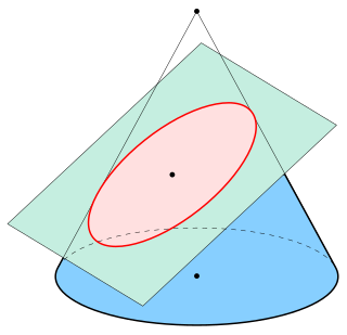
In mathematics, an ellipse is a plane curve surrounding two focal points, such that for all points on the curve, the sum of the two distances to the focal points is a constant. It generalizes a circle, which is the special type of ellipse in which the two focal points are the same. The elongation of an ellipse is measured by its eccentricity , a number ranging from to .

<span class="mw-page-title-main">Cardioid</span> Type of plane curve

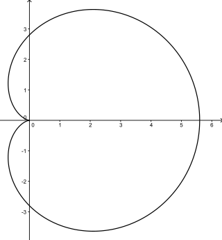
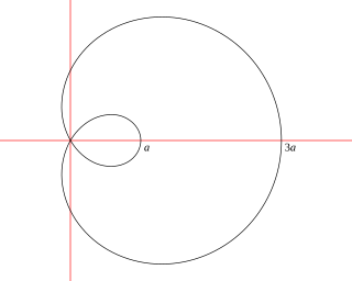
In geometry, a cardioid is a plane curve traced by a point on the perimeter of a circle that is rolling around a fixed circle of the same radius. It can also be defined as an epicycloid having a single cusp. It is also a type of sinusoidal spiral, and an inverse curve of the parabola with the focus as the center of inversion. A cardioid can also be defined as the set of points of reflections of a fixed point on a circle through all tangents to the circle.

<span class="mw-page-title-main">Epicycloid</span> Plane curve traced by a point on a circle rolled around another circle

In geometry, an epicycloid(also called hypercycloid) is a plane curve produced by tracing the path of a chosen point on the circumference of a circle—called an epicycle—which rolls without slipping around a fixed circle. It is a particular kind of roulette.

<span class="mw-page-title-main">Bloch sphere</span> Geometrical representation of the pure state space of a two-level quantum mechanical system

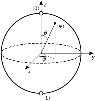
In quantum mechanics and computing, the Bloch sphere is a geometrical representation of the pure state space of a two-level quantum mechanical system (qubit), named after the physicist Felix Bloch.

<span class="mw-page-title-main">Cissoid of Diocles</span> Cubic plane curve

In geometry, the cissoid of Diocles is a cubic plane curve notable for the property that it can be used to construct two mean proportionals to a given ratio. In particular, it can be used to double a cube. It can be defined as the cissoid of a circle and a line tangent to it with respect to the point on the circle opposite to the point of tangency. In fact, the curve family of cissoids is named for this example and some authors refer to it simply as the cissoid. It has a single cusp at the pole, and is symmetric about the diameter of the circle which is the line of tangency of the cusp. The line is an asymptote. It is a member of the conchoid of de Sluze family of curves and in form it resembles a tractrix.

<span class="mw-page-title-main">Involute</span> Curve traced by a string as it is unwrapped from another curve

In mathematics, an involute is a particular type of curve that is dependent on another shape or curve. An involute of a curve is the locus of a point on a piece of taut string as the string is either unwrapped from or wrapped around the curve.

<span class="mw-page-title-main">Nephroid</span> Plane curve; an epicycloid with radii differing by 1/2

In geometry, a nephroid is a specific plane curve. It is a type of epicycloid in which the smaller circle's radius differs from the larger one by a factor of one-half.

<span class="mw-page-title-main">Envelope (mathematics)</span> Family of curves in geometry

In geometry, an envelope of a planar family of curves is a curve that is tangent to each member of the family at some point, and these points of tangency together form the whole envelope. Classically, a point on the envelope can be thought of as the intersection of two "infinitesimally adjacent" curves, meaning the limit of intersections of nearby curves. This idea can be generalized to an envelope of surfaces in space, and so on to higher dimensions.

<span class="mw-page-title-main">Cissoid</span> Plane curve constructed from two other curves and a fixed point

In geometry, a cissoid ( is a plane curve generated from two given curves C1, C2 and a point O. Let L be a variable line passing through O and intersecting C1 at P1 and C2 at P2. Let P be the point on L so that Then the locus of such points P is defined to be the cissoid of the curves C1, C2 relative to O.

<span class="mw-page-title-main">Tangent half-angle formula</span> Relates the tangent of half of an angle to trigonometric functions of the entire angle

In trigonometry, tangent half-angle formulas relate the tangent of half of an angle to trigonometric functions of the entire angle. The tangent of half an angle is the stereographic projection of the circle onto a line. Among these formulas are the following:

<span class="mw-page-title-main">Osculating circle</span> Circle of immediate corresponding curvature of a curve at a point

In differential geometry of curves, the osculating circle of a sufficiently smooth plane curve at a given point p on the curve has been traditionally defined as the circle passing through p and a pair of additional points on the curve infinitesimally close to p. Its center lies on the inner normal line, and its curvature defines the curvature of the given curve at that point. This circle, which is the one among all tangent circles at the given point that approaches the curve most tightly, was named circulus osculans by Leibniz.

<span class="mw-page-title-main">Strophoid</span> Geometric curve constructed from another curve and two points

In geometry, a strophoid is a curve generated from a given curve C and points A and O as follows: Let L be a variable line passing through O and intersecting C at K. Now let P1 and P2 be the two points on L whose distance from K is the same as the distance from A to K. The locus of such points P1 and P2 is then the strophoid of C with respect to the pole O and fixed point A. Note that AP1 and AP2 are at right angles in this construction.

<span class="mw-page-title-main">Watt's curve</span> Algebraic curve

In mathematics, Watt's curve is a tricircular plane algebraic curve of degree six. It is generated by two circles of radius b with centers distance 2a apart. A line segment of length 2c attaches to a point on each of the circles, and the midpoint of the line segment traces out the Watt curve as the circles rotate partially back and forth or completely around. It arose in connection with James Watt's pioneering work on the steam engine.

There are several equivalent ways for defining trigonometric functions, and the proof of the trigonometric identities between them depend on the chosen definition. The oldest and somehow the most elementary definition is based on the geometry of right triangles. The proofs given in this article use this definition, and thus apply to non-negative angles not greater than a right angle. For greater and negative angles, see Trigonometric functions.

<span class="mw-page-title-main">Gravitational lensing formalism</span>

In general relativity, a point mass deflects a light ray with impact parameter by an angle approximately equal to

<span class="mw-page-title-main">Limaçon trisectrix</span> Quartic plane curve

In geometry, a limaçon trisectrix is the name for the quartic plane curve that is a trisectrix that is specified as a limaçon. The shape of the limaçon trisectrix can be specified by other curves particularly as a rose, conchoid or epitrochoid. The curve is one among a number of plane curve trisectrixes that includes the Conchoid of Nicomedes, the Cycloid of Ceva, Quadratrix of Hippias, Trisectrix of Maclaurin, and Tschirnhausen cubic. The limaçon trisectrix a special case of a sectrix of Maclaurin.

<span class="mw-page-title-main">Sectrix of Maclaurin</span> Curve traced by the crossing of two lines revolving about poles

In geometry, a sectrix of Maclaurin is defined as the curve swept out by the point of intersection of two lines which are each revolving at constant rates about different points called poles. Equivalently, a sectrix of Maclaurin can be defined as a curve whose equation in biangular coordinates is linear. The name is derived from the trisectrix of Maclaurin, which is a prominent member of the family, and their sectrix property, which means they can be used to divide an angle into a given number of equal parts. There are special cases known as arachnida or araneidans because of their spider-like shape, and Plateau curves after Joseph Plateau who studied them.

<span class="mw-page-title-main">Law of cosines</span> Property of all triangles on a Euclidean plane

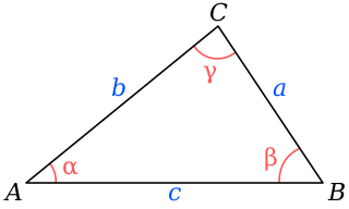
In trigonometry, the law of cosines relates the lengths of the sides of a triangle to the cosine of one of its angles. For a triangle with sides and opposite respective angles and , the law of cosines states:

For a plane curve C and a given fixed point O, the pedal equation of the curve is a relation between r and p where r is the distance from O to a point on C and p is the perpendicular distance from O to the tangent line to C at the point. The point O is called the pedal point and the values r and p are sometimes called the pedal coordinates of a point relative to the curve and the pedal point. It is also useful to measure the distance of O to the normal even though it is not an independent quantity and it relates to as .

References

Notes

  1. Edwards p. 165
  2. Edwards p. 164
  3. Follows Edwards p. 164 with m=1
  4. Edwards p. 164-5
  5. Follows Edwards p. 165 with m=1
  6. Williamson p. 228
  7. Edwards p. 167

Sources

Further reading