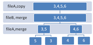
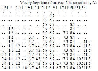
Block sort stably sorting numbers 1 to 16. Insertion sort groups of 16, extract two internal buffers, tag the A blocks (of size √16 = 4 each), roll the A blocks through B, locally merge them, sort the second buffer, and redistribute the buffers.
Block sort, or block merge sort, is a sorting algorithm combining at least two merge operations with an insertion sort to arrive at O(n log n) (see Big O notation) in-placestable sorting time. It gets its name from the observation that merging two sorted lists, A and B, is equivalent to breaking A into evenly sized blocks, inserting each A block into B under special rules, and merging AB pairs.
One practical algorithm for O(n log n) in-place merging was proposed by Pok-Son Kim and Arne Kutzner in 2008.[1]
Overview
The outer loop of block sort is identical to a bottom-up merge sort, where each level of the sort merges pairs of subarrays, A and B, in sizes of 1, then 2, then 4, 8, 16, and so on, until both subarrays combined are the array itself.
Rather than merging A and B directly as with traditional methods, a block-based merge algorithm divides A into discrete blocks of size √A (resulting in √Anumber of blocks as well),[2] inserts each A block into B such that the first value of each A block is less than or equal (≤) to the B value immediately after it, then locally merges each A block with any B values between it and the next A block.
As merges still require a separate buffer large enough to hold the A block to be merged, two areas within the array are reserved for this purpose (known as internal buffers).[3] The first two A blocks are thus modified to contain the first instance of each value within A, with the original contents of those blocks shifted over if necessary. The remaining A blocks are then inserted into B and merged using one of the two buffers as swap space. This process causes the values in that buffer to be rearranged.
Once every A and B block of every A and B subarray have been merged for that level of the merge sort, the values in that buffer must be sorted to restore their original order, so an insertion sort must be applied. The values in the buffers are then redistributed to their first sorted position within the array. This process repeats for each level of the outer bottom-up merge sort, at which point the array will have been stably sorted.
Algorithm
The following operators are used in the code examples:
Additionally, block sort relies on the following operations as part of its overall algorithm:
Swap: exchange the positions of two values in an array.
Block swap: exchange a range of values within an array with values in a different range of the array.
Binary search: assuming the array is sorted, check the middle value of the current search range, then if the value is lesser check the lower range, and if the value is greater check the upper range. Block sort uses two variants: one which finds the first position to insert a value in the sorted array, and one which finds the last position.
Linear search: find a particular value in an array by checking every single element in order, until it is found.
Insertion sort: for each item in the array, loop backward and find where it needs to be inserted, then insert it at that position.
Array rotation: move the items in an array to the left or right by some number of spaces, with values on the edges wrapping around to the other side. Rotations can be implemented as three reversals.[4]
Floor power of two: floor a value to the next power of two. Thus 63 becomes 32, 64 stays 64, and so forth.[5]
FloorPowerOfTwo(x) x = x | (x >> 1) x = x | (x >> 2) x = x | (x >> 4) x = x | (x >> 8) x = x | (x >> 16) if (this is a 64-bit system) x = x | (x >> 32) return x - (x >> 1)
Outer loop
As previously stated, the outer loop of a block sort is identical to a bottom-up merge sort. However, it benefits from the variant that ensures each A and B subarray are the same size to within one item:
BlockSort(array) power_of_two = FloorPowerOfTwo(array.size) scale = array.size/power_of_two // 1.0 ≤ scale < 2.0// insertion sort 16–31 items at a timefor (merge = 0; merge < power_of_two; merge += 16) start = merge * scale end = start + 16 * scale InsertionSort(array, [start, end)) for (length = 16; length < power_of_two; length += length) for (merge = 0; merge < power_of_two; merge += length * 2) start = merge * scale mid = (merge + length) * scale end = (merge + length * 2) * scale if (array[end − 1] < array[start]) // the two ranges are in reverse order, so a rotation is enough to merge themRotate(array, mid − start, [start, end)) else if (array[mid − 1] > array[mid]) Merge(array, A = [start, mid), B = [mid, end)) // else the ranges are already correctly ordered
Fixed-point math may also be used, by representing the scale factor as a fraction integer_part + numerator/denominator:
BlockSort(array) power_of_two = FloorPowerOfTwo(array.size) denominator = power_of_two/16 numerator_step = array.size % denominator integer_step = floor(array.size/denominator) // insertion sort 16–31 items at a timewhile (integer_step < array.size) integer_part = numerator = 0 while (integer_part < array.size) // get the ranges for A and B start = integer_part integer_part += integer_step numerator += numerator_step if (numerator ≥ denominator) numerator −= denominator integer_part++ mid = integer_part integer_part += integer_step numerator += numerator_step if (numerator ≥ denominator) numerator −= denominator integer_part++ end = integer_part if (array[end − 1] < array[start]) Rotate(array, mid − start, [start, end)) else if (array[mid − 1] > array[mid]) Merge(array, A = [start, mid), B = [mid, end)) integer_step += integer_step numerator_step += numerator_step if (numerator_step ≥ denominator) numerator_step −= denominator integer_step++
Extract buffers
The buffer extraction process for block sort.
The two internal buffers needed for each level of the merge step are created by moving the first 2√A first instances of their values within an A subarray to the start of A. First it iterates over the elements in A and counts off the unique values it needs, then it applies array rotations to move those unique values to the start.[6] If A did not contain enough unique values to fill the two buffers (of size √A each), B can be used just as well. In this case it moves the last instance of each value to the end of B, with that part of B not being included during the merges.
while (integer_step < array.size) block_size = √integer_step buffer_size = integer_step/block_size + 1 [extract two buffers of size 'buffer_size' each]
If B does not contain enough unique values either, it pulls out the largest number of unique values it could find, then adjusts the size of the A and B blocks such that the number of resulting A blocks is less than or equal to the number of unique items pulled out for the buffer. Only one buffer will be used in this case – the second buffer won't exist.
buffer_size = [number of unique values found] block_size = integer_step/buffer_size + 1 integer_part = numerator = 0 while (integer_part < array.size) [get the ranges for A and B][adjust A and B to not include the ranges used by the buffers]
Tag A blocks
Tagging the A blocks using values from the first internal buffer. Note that the first A block and last B block are unevenly sized.
Once the one or two internal buffers have been created, it begins merging each A and B subarray for this level of the merge sort. To do so, it divides each A and B subarray into evenly sized blocks of the size calculated in the previous step, where the first A block and last B block are unevenly sized if needed. It then loops over each of the evenly sized A blocks and swaps the second value with a corresponding value from the first of the two internal buffers. This is known as tagging the blocks.
// blockA is the range of the remaining A blocks,// and firstA is the unevenly sized first A block blockA = [A.start, A.end) firstA = [A.start, A.start + |blockA| % block_size) // swap the second value of each A block with the value in buffer1for (index = 0, indexA = firstA.end + 1; indexA < blockA.end; indexA += block_size) Swap(array[buffer1.start + index], array[indexA]) index++ lastA = firstA blockB = [B.start, B.start + minimum(block_size, |B|)) blockA.start += |firstA|
Roll and drop
Two A blocks rolling through the B blocks. Once the first A block is dropped behind, the unevenly sized A block is locally merged with the B values that follow it.
After defining and tagging the A blocks in this manner, the A blocks are rolled through the B blocks by block swapping the first evenly sized A block with the next B block. This process repeats until the first value of the A block with the smallest tag value is less than or equal to the last value of the B block that was just swapped with an A block.
At that point, the minimum A block (the A block with the smallest tag value) is swapped to the start of the rolling A blocks and the tagged value is restored with its original value from the first buffer. This is known as dropping a block behind, as it will no longer be rolled along with the remaining A blocks. That A block is then inserted into the previous B block, first by using a binary search on B to find the index where the first value of A is less than or equal to the value at that index of B, and then by rotating A into B at that index.
minA = blockA.start indexA = 0 while (true) // if there's a previous B block and the first value of the minimum A block is ≤// the last value of the previous B block, then drop that minimum A block behind.// or if there are no B blocks left then keep dropping the remaining A blocks.if ((|lastB| > 0 and array[lastB.end - 1] ≥ array[minA]) or |blockB| = 0) // figure out where to split the previous B block, and rotate it at the split B_split = BinaryFirst(array, array[minA], lastB) B_remaining = lastB.end - B_split // swap the minimum A block to the beginning of the rolling A blocksBlockSwap(array, blockA.start, minA, block_size) // restore the second value for the A blockSwap(array[blockA.start + 1], array[buffer1.start + indexA]) indexA++ // rotate the A block into the previous B blockRotate(array, blockA.start - B_split, [B_split, blockA.start + block_size)) // locally merge the previous A block with the B values that follow it,// using the second internal buffer as swap space (if it exists)if (|buffer2| > 0) MergeInternal(array, lastA, [lastA.end, B_split), buffer2) elseMergeInPlace(array, lastA, [lastA.end, B_split)) // update the range for the remaining A blocks,// and the range remaining from the B block after it was split lastA = [blockA.start - B_remaining, blockA.start - B_remaining + block_size) lastB = [lastA.end, lastA.end + B_remaining) // if there are no more A blocks remaining, this step is finished blockA.start = blockA.start + block_size if (|blockA| = 0) break minA = [new minimum A block](see below)else if (|blockB| < block_size) // move the last B block, which is unevenly sized,// to before the remaining A blocks, by using a rotationRotate(array, blockB.start - blockA.start, [blockA.start, blockB.end)) lastB = [blockA.start, blockA.start + |blockB|) blockA.start += |blockB| blockA.end += |blockB| minA += |blockB| blockB.end = blockB.start else// roll the leftmost A block to the end by swapping it with the next B blockBlockSwap(array, blockA.start, blockB.start, block_size) lastB = [blockA.start, blockA.start + block_size) if (minA = blockA.start) minA = blockA.end blockA.start += block_size blockA.end += block_size blockB.start += block_size // this is equivalent to minimum(blockB.end + block_size, B.end),// but that has the potential to overflowif (blockB.end > B.end - block_size) blockB.end = B.end else blockB.end += block_size // merge the last A block with the remaining B valuesif (|buffer2| > 0) MergeInternal(array, lastA, [lastA.end, B.end), buffer2) elseMergeInPlace(array, lastA, [lastA.end, B.end))
One optimization that can be applied during this step is the floating-hole technique.[7] When the minimum A block is dropped behind and needs to be rotated into the previous B block, after which its contents are swapped into the second internal buffer for the local merges, it would be faster to swap the A block to the buffer beforehand, and to take advantage of the fact that the contents of that buffer do not need to retain any order. So rather than rotating the second buffer (which used to be the A block before the block swap) into the previous B block at position index, the values in the B block after index can simply be block swapped with the last items of the buffer.
The floating hole in this case refers to the contents of the second internal buffer floating around the array, and acting as a hole in the sense that the items do not need to retain their order.
Local merges
Once the A block has been rotated into the B block, the previous A block is then merged with the B values that follow it, using the second buffer as swap space. When the first A block is dropped behind this refers to the unevenly sized A block at the start, when the second A block is dropped behind it means the first A block, and so forth.
MergeInternal(array, A, B, buffer) // block swap the values in A with those in 'buffer'BlockSwap(array, A.start, buffer.start, |A|) A_count = 0, B_count = 0, insert = 0 while (A_count < |A| and B_count < |B|) if (array[buffer.start + A_count] ≤ array[B.start + B_count]) Swap(array[A.start + insert], array[buffer.start + A_count]) A_count++ elseSwap(array[A.start + insert], array[B.start + B_count]) B_count++ insert++ // block swap the remaining part of the buffer with the remaining part of the arrayBlockSwap(array, buffer.start + A_count, A.start + insert, |A| - A_count)
If the second buffer does not exist, a strictly in-place merge operation must be performed, such as a rotation-based version of the Hwang and Lin algorithm,[7][8] the Dudzinski and Dydek algorithm,[9] or a repeated binary search and rotate.
MergeInPlace(array, A, B) while (|A| > 0 and |B| > 0) // find the first place in B where the first item in A needs to be inserted mid = BinaryFirst(array, array[A.start], B) // rotate A into place amount = mid - A.end Rotate(array, amount, [A.start, mid)) // calculate the new A and B ranges B = [mid, B.end) A = [A.start + amount, mid) A.start = BinaryLast(array, array[A.start], A)
After dropping the minimum A block and merging the previous A block with the B values that follow it, the new minimum A block must be found within the blocks that are still being rolled through the array. This is handled by running a linear search through those A blocks and comparing the tag values to find the smallest one.
minA = blockA.start for (findA = minA + block_size; findA < blockA.end - 1; findA += block_size) if (array[findA + 1] < array[minA + 1]) minA = findA
These remaining A blocks then continue rolling through the array and being dropped and inserted where they belong. This process repeats until all of the A blocks have been dropped and rotated into the previous B block.
Once the last remaining A block has been dropped behind and inserted into B where it belongs, it should be merged with the remaining B values that follow it. This completes the merge process for that particular pair of A and B subarrays. However, it must then repeat the process for the remaining A and B subarrays for the current level of the merge sort.
Note that the internal buffers can be reused for every set of A and B subarrays for this level of the merge sort, and do not need to be re-extracted or modified in any way.
Redistribute
After all of the A and B subarrays have been merged, the one or two internal buffers are still left over. The first internal buffer was used for tagging the A blocks, and its contents are still in the same order as before, but the second internal buffer may have had its contents rearranged when it was used as swap space for the merges. This means the contents of the second buffer will need to be sorted using a different algorithm, such as insertion sort. The two buffers must then be redistributed back into the array using the opposite process that was used to create them.
After repeating these steps for every level of the bottom-up merge sort, the block sort is completed.
Variants
Block sort works by extracting two internal buffers, breaking A and B subarrays into evenly sized blocks, rolling and dropping the A blocks into B (using the first buffer to track the order of the A blocks), locally merging using the second buffer as swap space, sorting the second buffer, and redistributing both buffers. While the steps do not change, these subsystems can vary in their actual implementation.
One variant of block sort allows it to use any amount of additional memory provided to it, by using this external buffer for merging an A subarray or A block with B whenever A fits into it. In this situation it would be identical to a merge sort.
Good choices for the buffer size include:
Size
Notes
(count + 1)/2
turns into a full-speed merge sort since all of the A subarrays will fit into it
√(count + 1)/2 + 1
this will be the size of the A blocks at the largest level of merges, so block sort can skip using internal or in-place merges for anything
512
a fixed-size buffer large enough to handle the numerous merges at the smaller levels of the merge sort
0
if the system cannot allocate any extra memory, no memory works well
Rather than tagging the A blocks using the contents of one of the internal buffers, an indirect movement-imitation buffer can be used instead.[1][10] This is an internal buffer defined as s1 t s2, where s1 and s2 are each as large as the number of A and B blocks, and t contains any values immediately following s1 that are equal to the last value of s1 (thus ensuring that no value in s2 appears in s1). A second internal buffer containing √A unique values is still used. The first √A values of s1 and s2 are then swapped with each other to encode information into the buffer about which blocks are A blocks and which are B blocks. When an A block at index i is swapped with a B block at index j (where the first evenly sized A block is initially at index 0), s1[i] and s1[j] are swapped with s2[i] and s2[j], respectively. This imitates the movements of the A blocks through B. The unique values in the second buffer are used to determine the original order of the A blocks as they are rolled through the B blocks. Once all of the A blocks have been dropped, the movement-imitation buffer is used to decode whether a given block in the array is an A block or a B block, each A block is rotated into B, and the second internal buffer is used as swap space for the local merges.
The second value of each A block doesn't necessarily need to be tagged – the first, last, or any other element could be used instead. However, if the first value is tagged, the values will need to be read from the first internal buffer (where they were swapped) when deciding where to drop the minimum A block.
Many sorting algorithms can be used to sort the contents of the second internal buffer, including unstable sorts like quicksort, since the contents of the buffer are guaranteed to be unique. Insertion sort is still recommended, though, for its situational performance and lack of recursion.
Wikisort, Mike McFadden's implementation based on Kutzner and Kim's paper.[12]
GrailSort (and the rewritten HolyGrailSort), Andrey Astrelin's implementation based on Huang and Langston (1992),[13] which ultimately describes a very similar algorithm.[14]
Analysis
Block sort is a well-defined and testable class of algorithms, with working implementations available as a merge and as a sort.[11][15][12] This allows its characteristics to be measured and considered.
Block sort begins by performing insertion sort on groups of 16–31 items in the array. Insertion sort is an operation, so this leads to anywhere from to , which is once the constant factors are omitted. It must also apply an insertion sort on the second internal buffer after each level of merging is completed. However, as this buffer was limited to in size, the operation also ends up being .
Next it must extract two internal buffers for each level of the merge sort. It does so by iterating over the items in the A and B subarrays and incrementing a counter whenever the value changes, and upon finding enough values it rotates them to the start of A or the end of B. In the worst case this will end up searching the entire array before finding non-contiguous unique values, which requires comparisons and rotations for values. This resolves to , or .
When none of the A or B subarrays contained unique values to create the internal buffers, a normally suboptimal in-place merge operation is performed where it repeatedly binary searches and rotates A into B. However, the known lack of unique values within any of the subarrays places a hard limit on the number of binary searches and rotations that will be performed during this step, which is again items rotated up to times, or . The size of each block is also adjusted to be smaller in the case where it found unique values but not 2, which further limits the number of unique values contained within any A or B block.
Tagging the A blocks is performed times for each A subarray, then the A blocks are rolled through and inserted into the B blocks up to times. The local merges retain the same complexity of a standard merge, albeit with more assignments since the values must be swapped rather than copied. The linear search for finding the new minimum A block iterates over blocks times. And the buffer redistribution process is identical to the buffer extraction but in reverse, and therefore has the same complexity.
After omitting all but the highest complexity and considering that there are levels in the outer merge loop, this leads to a final asymptotic complexity of for the worst and average cases. For the best case, where the data is already in order, the merge step performs comparisons for the first level, then , , , etc. This is a well-known mathematical series which resolves to .
Memory
As block sort is non-recursive and does not require the use of dynamic allocations, this leads to constant stack and heap space. It uses O(1) auxiliary memory in a transdichotomous model, which accepts that the O(log n) bits needed to keep track of the ranges for A and B cannot be any greater than 32 or 64 on 32-bit or 64-bit computing systems, respectively, and therefore simplifies to O(1) space for any array that can feasibly be allocated.
Although items in the array are moved out of order during a block sort, each operation is fully reversible and will have restored the original order of equivalent items by its completion.
Stability requires the first instance of each value in an array before sorting to still be the first instance of that value after sorting. Block sort moves these first instances to the start of the array to create the two internal buffers, but when all of the merges are completed for the current level of the block sort, those values are distributed back to the first sorted position within the array. This maintains stability.
Before rolling the A blocks through the B blocks, each A block has its second value swapped with a value from the first buffer. At that point the A blocks are moved out of order to roll through the B blocks. However, once it finds where it should insert the smallest A block into the previous B block, that smallest A block is moved back to the start of the A blocks and its second value is restored. By the time all of the A blocks have been inserted, the A blocks will be in order again and the first buffer will contain its original values in the original order.
Using the second buffer as swap space when merging an A block with some B values causes the contents of that buffer to be rearranged. However, as the algorithm already ensured the buffer only contains unique values, sorting the contents of the buffer is sufficient to restore their original stable order.
Adaptivity
Block sort is an adaptive sort on two levels: first, it skips merging A and B subarrays that are already in order. Next, when A and B need to be merged and are broken into evenly sized blocks, the A blocks are only rolled through B as far as is necessary, and each block is only merged with the B values immediately following it. The more ordered the data originally was, the fewer B values there will be that need to be merged into A.
Advantages
Block sort is a stable sort that does not require additional memory, which is useful in cases where there is not enough free memory to allocate the O(n) buffer. When using the external buffer variant of block sort, it can scale from using O(n) memory to progressively smaller buffers as needed, and will still work efficiently within those constraints.
Disadvantages
Block sort does not exploit sorted ranges of data on as fine a level as some other algorithms, such as Timsort.[16] It only checks for these sorted ranges at the two predefined levels: the A and B subarrays, and the A and B blocks. It is also harder to implement and parallelize compared to a merge sort.
Related Research Articles
In computer science, merge sort is an efficient, general-purpose, and comparison-based sorting algorithm. Most implementations produce a stable sort, which means that the relative order of equal elements is the same in the input and output. Merge sort is a divide-and-conquer algorithm that was invented by John von Neumann in 1945. A detailed description and analysis of bottom-up merge sort appeared in a report by Goldstine and von Neumann as early as 1948.
In computer science, radix sort is a non-comparative sorting algorithm. It avoids comparison by creating and distributing elements into buckets according to their radix. For elements with more than one significant digit, this bucketing process is repeated for each digit, while preserving the ordering of the prior step, until all digits have been considered. For this reason, radix sort has also been called bucket sort and digital sort.
In computer science, a sorting algorithm is an algorithm that puts elements of a list into an order. The most frequently used orders are numerical order and lexicographical order, and either ascending or descending. Efficient sorting is important for optimizing the efficiency of other algorithms that require input data to be in sorted lists. Sorting is also often useful for canonicalizing data and for producing human-readable output.
A binary heap is a heap data structure that takes the form of a binary tree. Binary heaps are a common way of implementing priority queues. The binary heap was introduced by J. W. J. Williams in 1964, as a data structure for heapsort.
Shellsort, also known as Shell sort or Shell's method, is an in-place comparison sort. It can be seen as either a generalization of sorting by exchange or sorting by insertion. The method starts by sorting pairs of elements far apart from each other, then progressively reducing the gap between elements to be compared. By starting with far-apart elements, it can move some out-of-place elements into the position faster than a simple nearest-neighbor exchange. Donald Shell published the first version of this sort in 1959. The running time of Shellsort is heavily dependent on the gap sequence it uses. For many practical variants, determining their time complexity remains an open problem.
Bucket sort, or bin sort, is a sorting algorithm that works by distributing the elements of an array into a number of buckets. Each bucket is then sorted individually, either using a different sorting algorithm, or by recursively applying the bucket sorting algorithm. It is a distribution sort, a generalization of pigeonhole sort that allows multiple keys per bucket, and is a cousin of radix sort in the most-to-least significant digit flavor. Bucket sort can be implemented with comparisons and therefore can also be considered a comparison sort algorithm. The computational complexity depends on the algorithm used to sort each bucket, the number of buckets to use, and whether the input is uniformly distributed.
In computer science, counting sort is an algorithm for sorting a collection of objects according to keys that are small positive integers; that is, it is an integer sorting algorithm. It operates by counting the number of objects that possess distinct key values, and applying prefix sum on those counts to determine the positions of each key value in the output sequence. Its running time is linear in the number of items and the difference between the maximum key value and the minimum key value, so it is only suitable for direct use in situations where the variation in keys is not significantly greater than the number of items. It is often used as a subroutine in radix sort, another sorting algorithm, which can handle larger keys more efficiently.
In computer science, the treap and the randomized binary search tree are two closely related forms of binary search tree data structures that maintain a dynamic set of ordered keys and allow binary searches among the keys. After any sequence of insertions and deletions of keys, the shape of the tree is a random variable with the same probability distribution as a random binary tree; in particular, with high probability its height is proportional to the logarithm of the number of keys, so that each search, insertion, or deletion operation takes logarithmic time to perform.
In computer science, arbitrary-precision arithmetic, also called bignum arithmetic, multiple-precision arithmetic, or sometimes infinite-precision arithmetic, indicates that calculations are performed on numbers whose digits of precision are potentially limited only by the available memory of the host system. This contrasts with the faster fixed-precision arithmetic found in most arithmetic logic unit (ALU) hardware, which typically offers between 8 and 64 bits of precision.
External sorting is a class of sorting algorithms that can handle massive amounts of data. External sorting is required when the data being sorted do not fit into the main memory of a computing device and instead they must reside in the slower external memory, usually a disk drive. Thus, external sorting algorithms are external memory algorithms and thus applicable in the external memory model of computation.
Quicksort is an efficient, general-purpose sorting algorithm. Quicksort was developed by British computer scientist Tony Hoare in 1959 and published in 1961. It is still a commonly used algorithm for sorting. Overall, it is slightly faster than merge sort and heapsort for randomized data, particularly on larger distributions.
In statistics, the Kendall rank correlation coefficient, commonly referred to as Kendall's τ coefficient, is a statistic used to measure the ordinal association between two measured quantities. A τ test is a non-parametric hypothesis test for statistical dependence based on the τ coefficient. It is a measure of rank correlation: the similarity of the orderings of the data when ranked by each of the quantities. It is named after Maurice Kendall, who developed it in 1938, though Gustav Fechner had proposed a similar measure in the context of time series in 1897.
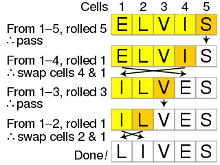
The Fisher–Yates shuffle is an algorithm for shuffling a finite sequence. The algorithm takes a list of all the elements of the sequence, and continually determines the next element in the shuffled sequence by randomly drawing an element from the list until no elements remain. The algorithm produces an unbiased permutation: every permutation is equally likely. The modern version of the algorithm takes time proportional to the number of items being shuffled and shuffles them in place.
Samplesort is a sorting algorithm that is a divide and conquer algorithm often used in parallel processing systems. Conventional divide and conquer sorting algorithms partitions the array into sub-intervals or buckets. The buckets are then sorted individually and then concatenated together. However, if the array is non-uniformly distributed, the performance of these sorting algorithms can be significantly throttled. Samplesort addresses this issue by selecting a sample of size s from the n-element sequence, and determining the range of the buckets by sorting the sample and choosing p−1 < s elements from the result. These elements then divide the array into p approximately equal-sized buckets. Samplesort is described in the 1970 paper, "Samplesort: A Sampling Approach to Minimal Storage Tree Sorting", by W. D. Frazer and A. C. McKellar.
ProxmapSort, or Proxmap sort, is a sorting algorithm that works by partitioning an array of data items, or keys, into a number of "subarrays". The name is short for computing a "proximity map," which indicates for each key K the beginning of a subarray where K will reside in the final sorted order. Keys are placed into each subarray using insertion sort. If keys are "well distributed" among the subarrays, sorting occurs in linear time. The computational complexity estimates involve the number of subarrays and the proximity mapping function, the "map key," used. It is a form of bucket and radix sort.
In computer science, a fractal tree index is a tree data structure that keeps data sorted and allows searches and sequential access in the same time as a B-tree but with insertions and deletions that are asymptotically faster than a B-tree. Like a B-tree, a fractal tree index is a generalization of a binary search tree in that a node can have more than two children. Furthermore, unlike a B-tree, a fractal tree index has buffers at each node, which allow insertions, deletions and other changes to be stored in intermediate locations. The goal of the buffers is to schedule disk writes so that each write performs a large amount of useful work, thereby avoiding the worst-case performance of B-trees, in which each disk write may change a small amount of data on disk. Like a B-tree, fractal tree indexes are optimized for systems that read and write large blocks of data. The fractal tree index has been commercialized in databases by Tokutek. Originally, it was implemented as a cache-oblivious lookahead array, but the current implementation is an extension of the Bε tree. The Bε is related to the Buffered Repository Tree. The Buffered Repository Tree has degree 2, whereas the Bε tree has degree Bε. The fractal tree index has also been used in a prototype filesystem. An open source implementation of the fractal tree index is available, which demonstrates the implementation details outlined below.
Heap's algorithm generates all possible permutations of n objects. It was first proposed by B. R. Heap in 1963. The algorithm minimizes movement: it generates each permutation from the previous one by interchanging a single pair of elements; the other n−2 elements are not disturbed. In a 1977 review of permutation-generating algorithms, Robert Sedgewick concluded that it was at that time the most effective algorithm for generating permutations by computer.
Funnelsort is a comparison-based sorting algorithm. It is similar to mergesort, but it is a cache-oblivious algorithm, designed for a setting where the number of elements to sort is too large to fit in a cache where operations are done. It was introduced by Matteo Frigo, Charles Leiserson, Harald Prokop, and Sridhar Ramachandran in 1999 in the context of the cache oblivious model.
The cache-oblivious distribution sort is a comparison-based sorting algorithm. It is similar to quicksort, but it is a cache-oblivious algorithm, designed for a setting where the number of elements to sort is too large to fit in a cache where operations are done. In the external memory model, the number of memory transfers it needs to perform a sort of items on a machine with cache of size and cache lines of length is , under the tall cache assumption that . This number of memory transfers has been shown to be asymptotically optimal for comparison sorts. This distribution sort also achieves the asymptotically optimal runtime complexity of .
Interpolation sort is a sorting algorithm that is a kind of bucket sort. It uses an interpolation formula to assign data to the bucket. A general interpolation formula is:
↑ Huang, B-C.; Langston, M. A. (1 December 1992). "Fast Stable Merging and Sorting in Constant Extra Space". The Computer Journal. 35 (6): 643–650. doi:10.1093/comjnl/35.6.643.
This page is based on this Wikipedia article Text is available under the CC BY-SA 4.0 license; additional terms may apply. Images, videos and audio are available under their respective licenses.