Smoothsort

Smoothsort

Smoothsort operating on an array which is mostly in order. The bars across the top show the tree structure.
Class	Sorting algorithm
Data structure	Array
Worst-case performance	O(n log n)
Best-case performance	O(n)
Average performance	O(n log n)
Worst-case space complexity	O(n) total, O(1) auxiliary
Optimal	When the data is already sorted

In computer science, smoothsort is a comparison-based sorting algorithm. A variant of heapsort, it was invented and published by Edsger Dijkstra in 1981. ^[1] Like heapsort, smoothsort is an in-place algorithm with an upper bound of O (n log n) operations (see big O notation), ^[2] but it is not a stable sort. ^{[3] [ self-published source? ] [4]} The advantage of smoothsort is that it comes closer to O(n) time if the input is already sorted to some degree, whereas heapsort averages O(n log n) regardless of the initial sorted state.

Overview

Like heapsort, smoothsort organizes the input into a priority queue and then repeatedly extracts the maximum. Also like heapsort, the priority queue is an implicit heap data structure (a heap-ordered implicit binary tree), which occupies a prefix of the array. Each extraction shrinks the prefix and adds the extracted element to a growing sorted suffix. When the prefix has shrunk to nothing, the array is completely sorted.

Heapsort maps the binary tree to the array using a top-down breadth-first traversal of the tree; the array begins with the root of the tree, then its two children, then four grandchildren, and so on. Every element has a well-defined depth below the root of the tree, and every element except the root has its parent earlier in the array. Its height above the leaves, however, depends on the size of the array. This has the disadvantage that every element must be moved as part of the sorting process: it must pass through the root before being moved to its final location.

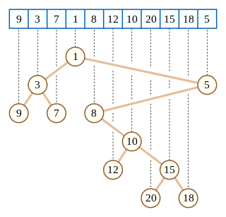
Smoothsort uses a different mapping, a bottom-up depth-first post-order traversal. A left child is followed by the subtree rooted at its sibling, and a right child is followed by its parent. Every element has a well-defined height above the leaves, and every non-leaf element has its children earlier in the array. Its depth below the root, however, depends on the size of the array. The algorithm is organized so the root is at the end of the heap, and at the moment that an element is extracted from the heap it is already in its final location and does not need to be moved. Also, a sorted array is already a valid heap, and many sorted intervals are valid heap-ordered subtrees.

More formally, every position i is the root of a unique subtree, whose nodes occupy a contiguous interval that ends at i. An initial prefix of the array (including the whole array), might be such an interval corresponding to a subtree, but in general decomposes as a union of a number of successive such subtree intervals, which Dijkstra calls "stretches". Any subtree without a parent (i.e. rooted at a position whose parent lies beyond the prefix under consideration) gives a stretch in the decomposition of that interval, which decomposition is therefore unique. When a new node is appended to the prefix, one of two cases occurs: either the position is a leaf and adds a stretch of length 1 to the decomposition, or it combines with the last two stretches, becoming the parent of their respective roots, thus replacing the two stretches by a new stretch containing their union plus the new (root) position.

Dijkstra noted ^[1] that the obvious rule would be to combine stretches if and only if they have equal size, in which case all subtrees would be perfect binary trees of size 2^k−1. However, he chose a different rule, which gives more possible tree sizes. This has the same asymptotic efficiency, ^[2] but gains a small constant factor in efficiency by requiring fewer stretches to cover each interval.

The rule Dijkstra uses is that the last two stretches are combined if and only if their sizes are consecutive Leonardo numbers L(i+1) and L(i) (in that order), which numbers are recursively defined, in a manner very similar to the Fibonacci numbers, as:

• L(0) = L(1) = 1
• L(k+2) = L(k+1) + L(k) + 1

As a consequence, the size of any subtree is a Leonardo number. The sequence of stretch sizes decomposing the first n positions, for any n, can be found in a greedy manner: the first size is the largest Leonardo number not exceeding n, and the remainder (if any) is decomposed recursively. The sizes of stretches are decreasing, strictly so except possibly for two final sizes 1, and avoiding successive Leonardo numbers except possibly for the final two sizes.

In addition to each stretch being a heap-ordered tree, the roots of the trees are maintained in sorted order. This effectively adds a third child (which Dijkstra calls a "stepson") to each root linking it to the preceding root. This combines all of the trees together into one global heap. with the global maximum at the end.

Although the location of each node's stepson is fixed, the link only exists for tree roots, meaning that links are removed whenever trees are merged. This is different from ordinary children, which are linked as long as the parent exists.

In the first (heap growing) phase of sorting, an increasingly large initial part of the array is reorganized so that the subtree for each of its stretches is a max-heap: the entry at any non-leaf position is at least as large as the entries at the positions that are its children. In addition, all roots are at least as large as their stepsons.

In the second (heap shrinking) phase, the maximal node is detached from the end of the array (without needing to move it) and the heap invariants are re-established among its children. (Specifically, among the newly created stepsons.)

Practical implementation frequently needs to compute Leonardo numbers L(k). Dijkstra provides clever code which uses a fixed number of integer variables to efficiently compute the values needed at the time they are needed. Alternatively, if there is a finite bound N on the size of arrays to be sorted, a precomputed table of Leonardo numbers can be stored in O(log N) space.

Operations

While the two phases of the sorting procedure are opposite to each other as far as the evolution of the sequence-of-heaps structure is concerned, they are implemented using one core primitive, equivalent to the "sift down" operation in a binary max-heap.

Sifting down

The core sift-down operation (which Dijkstra calls "trinkle") restores the heap invariant when it is possibly violated only at the root node. If the root node is less than any of its children, it is swapped with its greatest child and the process repeated with the root node in its new subtree.

The difference between smoothsort and a binary max-heap is that the root of each stretch must be ordered with respect to a third "stepson": the root of the preceding stretch. So the sift-down procedure starts with a series of four-way comparisons (the root node and three children) until the stepson is not the maximal element, then a series of three-way comparisons (the root plus two children) until the root node finds its final home and the invariants are re-established.

Each tree is a full binary tree: each node has two children or none. There is no need to deal with the special case of one child which occurs in a standard implicit binary heap. (But the special case of stepson links more than makes up for this saving.)

Because there are O(log n) stretches, each of which is a tree of depth O(log n), the time to perform each sifting-down operation is bounded by O(log n).

Growing the heap region by incorporating an element to the right

When an additional element is considered for incorporation into the sequence of stretches (list of disjoint heap structures) it either forms a new one-element stretch, or it combines the two rightmost stretches by becoming the parent of both their roots and forming a new stretch that replaces the two in the sequence. Which of the two happens depends only on the sizes of the stretches currently present (and ultimately only on the index of the element added); Dijkstra stipulated that stretches are combined if and only if their sizes are L(k+1) and L(k) for some k, i.e., consecutive Leonardo numbers; the new stretch will have size L(k+2).

In either case, the new element must be sifted down to its correct place in the heap structure. Even if the new node is a one-element stretch, it must still be sorted relative to the preceding stretch's root.

Optimization

Dijkstra's algorithm saves work by observing that the full heap invariant is required at the end of the growing phase, but it is not required at every intermediate step. In particular, the requirement that an element be greater than its stepson is only important for the elements which are the final tree roots.

Therefore, when an element is added, compute the position of its future parent. If this is within the range of remaining values to be sorted, act as if there is no stepson and only sift down within the current tree.

Shrinking the heap region by separating the rightmost element from it

During this phase, the form of the sequence of stretches goes through the changes of the growing phase in reverse. No work at all is needed when separating off a leaf node, but for a non-leaf node its two children become roots of new stretches, and need to be moved to their proper place in the sequence of roots of stretches. This can be obtained by applying sift-down twice: first for the left child, and then for the right child (whose stepson was the left child).

Because half of all nodes in a full binary tree are leaves, this performs an average of one sift-down operation per node.

Optimization

It is already known that the newly exposed roots are correctly ordered with respect to their normal children; it is only the ordering relative to their stepsons which is in question. Therefore, while shrinking the heap, the first step of sifting down can be simplified to a single comparison with the stepson. If a swap occurs, subsequent steps must do the full four-way comparison.

Analysis

Smoothsort takes O(n) time to process a presorted array, O(n log n) in the worst case, and achieves nearly linear performance on many nearly sorted inputs. However, it does not handle all nearly sorted sequences optimally. Using the count of inversions as a measure of un-sortedness (the number of pairs of indices i and j with i < j and A[i] > A[j]; for randomly sorted input this is approximately n²/4), there are possible input sequences with O(n log n) inversions which cause it to take Ω(n log n) time, whereas other adaptive sorting algorithms can solve these cases in O(n log log n) time. ^[2]

The smoothsort algorithm needs to be able to hold in memory the sizes of all of the trees in the Leonardo heap. Since they are sorted by order and all orders are distinct, this is usually done using a bit vector indicating which orders are present. Moreover, since the largest order is at most O(log n), these bits can be encoded in O(1) machine words, assuming a transdichotomous machine model.

Note that O(1) machine words is not the same thing as one machine word. A 32-bit vector would only suffice for sizes less than L(32) = 7049155. A 64-bit vector will do for sizes less than L(64) = 34335360355129 ≈ 2⁴⁵. In general, it takes 1/log₂( φ ) ≈ 1.44 bits of vector per bit of size.

Poplar sort

A simpler algorithm inspired by smoothsort is poplar sort. ^[5] Named after the rows of trees of decreasing size often seen in Dutch polders, it performs fewer comparisons than smoothsort for inputs that are not mostly sorted, but cannot achieve linear time for sorted inputs.

The significant change made by poplar sort in that the roots of the various trees are not kept in sorted order; there are no "stepson" links tying them together into a single heap. Instead, each time the heap is shrunk in the second phase, the roots are searched to find the maximum entry.

Because there are n shrinking steps, each of which must search O(log n) tree roots for the maximum, the best-case run time for poplar sort is O(n log n).

The authors also suggest using perfect binary trees rather than Leonardo trees to provide further simplification, but this is a less significant change.

The same structure has been proposed as a general-purpose priority queue under the name post-order heap, ^[6] achieving O(1) amortized insertion time in a structure simpler than an implicit binomial heap.

Applications

The musl C library uses smoothsort for its implementation of qsort(). ^{[7] [8]}

References

1. Dijkstra, Edsger W. 16 Aug 1981 (EWD-796a) (PDF). E.W. Dijkstra Archive. Center for American History, University of Texas at Austin. One can also raise the question why I have not chosen as available stretch lengths: ... 63 31 15 7 3 1 which seems attractive since each stretch can then be viewed as the postorder traversal of a balanced binary tree. In addition, the recurrence relation would be simpler. But I know why I chose the Leonardo numbers: ( transcription )
2. Hertel, Stefan (13 May 1983). "Smoothsort's behavior on presorted sequences" (PDF). Information Processing Letters . 16 (4): 165–170. doi:10.1016/0020-0190(83)90116-3. Archived (PDF) from the original on 2015-12-08.
3. Brown, Craig (21 Jan 2013). "Fastest In-Place Stable Sort". Code Project.^{[ self-published source ]}
4. Eisenstat, David (13 September 2020). "Where is the smoothsort algorithm used?". Stack Overflow. Retrieved 2020-10-28. Smoothsort is not stable, and stability is often more desirable than in-place in practice
5. Bron, Coenraad; Hesselink, Wim H. (13 September 1991). "Smoothsort revisited". Information Processing Letters. 39 (5): 269–276. doi:10.1016/0020-0190(91)90027-F.
6. Harvey, Nicholas J. A.; Zatloukal, Kevin (26–28 May 2004). The Post-Order Heap. Third International Conference on Fun with Algorithms (FUN 2004). Elba, Italy.
7. Felker, Rich (30 April 2013). "How do different languages implement sorting in their standard libraries?". Stack Overflow. Retrieved 2020-10-28.
8. Ochs, Lynn; Felker, Rich (11 August 2017). "src/stdlib/qsort.c". musl - an implementation of the standard library for Linux-based systems. Retrieved 2021-01-26.

External links

• Commented transcription of EWD796a, 16-Aug-1981
• Detailed modern explanation of Smoothsort
• wikibooks:Algorithm Implementation/Sorting/Smoothsort
• Description and example implementation of Poplar heap
• Noshita, Kohei; Nakatani, Yoshinobu (April 1985). "On the Nested Heap Structure in Smoothsort". Mathematical Foundations of Computer Science and Their Applications (Japanese: 数理解析研究所講究録). 556: 1–16. hdl:2433/98975.