Related Research Articles
In computer science, heapsort is a comparison-based sorting algorithm. Heapsort can be thought of as an improved selection sort: like selection sort, heapsort divides its input into a sorted and an unsorted region, and it iteratively shrinks the unsorted region by extracting the largest element from it and inserting it into the sorted region. Unlike selection sort, heapsort does not waste time with a linear-time scan of the unsorted region; rather, heap sort maintains the unsorted region in a heap data structure to more quickly find the largest element in each step.
Insertion sort is a simple sorting algorithm that builds the final sorted array (or list) one item at a time by comparisons. It is much less efficient on large lists than more advanced algorithms such as quicksort, heapsort, or merge sort. However, insertion sort provides several advantages:
In computer science, merge sort is an efficient, general-purpose, and comparison-based sorting algorithm. Most implementations produce a stable sort, which means that the relative order of equal elements is the same in the input and output. Merge sort is a divide-and-conquer algorithm that was invented by John von Neumann in 1945. A detailed description and analysis of bottom-up merge sort appeared in a report by Goldstine and von Neumann as early as 1948.
In computer science, radix sort is a non-comparative sorting algorithm. It avoids comparison by creating and distributing elements into buckets according to their radix. For elements with more than one significant digit, this bucketing process is repeated for each digit, while preserving the ordering of the prior step, until all digits have been considered. For this reason, radix sort has also been called bucket sort and digital sort.

In computer science, a sorting algorithm is an algorithm that puts elements of a list into an order. The most frequently used orders are numerical order and lexicographical order, and either ascending or descending. Efficient sorting is important for optimizing the efficiency of other algorithms that require input data to be in sorted lists. Sorting is also often useful for canonicalizing data and for producing human-readable output.
In computer science, best, worst, and average cases of a given algorithm express what the resource usage is at least, at most and on average, respectively. Usually the resource being considered is running time, i.e. time complexity, but could also be memory or some other resource. Best case is the function which performs the minimum number of steps on input data of n elements. Worst case is the function which performs the maximum number of steps on input data of size n. Average case is the function which performs an average number of steps on input data of n elements.

Bucket sort, or bin sort, is a sorting algorithm that works by distributing the elements of an array into a number of buckets. Each bucket is then sorted individually, either using a different sorting algorithm, or by recursively applying the bucket sorting algorithm. It is a distribution sort, a generalization of pigeonhole sort that allows multiple keys per bucket, and is a cousin of radix sort in the most-to-least significant digit flavor. Bucket sort can be implemented with comparisons and therefore can also be considered a comparison sort algorithm. The computational complexity depends on the algorithm used to sort each bucket, the number of buckets to use, and whether the input is uniformly distributed.
In computer science, counting sort is an algorithm for sorting a collection of objects according to keys that are small positive integers; that is, it is an integer sorting algorithm. It operates by counting the number of objects that possess distinct key values, and applying prefix sum on those counts to determine the positions of each key value in the output sequence. Its running time is linear in the number of items and the difference between the maximum key value and the minimum key value, so it is only suitable for direct use in situations where the variation in keys is not significantly greater than the number of items. It is often used as a subroutine in radix sort, another sorting algorithm, which can handle larger keys more efficiently.

Cocktail shaker sort, also known as bidirectional bubble sort, cocktail sort, shaker sort, ripple sort, shuffle sort, or shuttle sort, is an extension of bubble sort. The algorithm extends bubble sort by operating in two directions. While it improves on bubble sort by more quickly moving items to the beginning of the list, it provides only marginal performance improvements.
Introsort or introspective sort is a hybrid sorting algorithm that provides both fast average performance and (asymptotically) optimal worst-case performance. It begins with quicksort, it switches to heapsort when the recursion depth exceeds a level based on (the logarithm of) the number of elements being sorted and it switches to insertion sort when the number of elements is below some threshold. This combines the good parts of the three algorithms, with practical performance comparable to quicksort on typical data sets and worst-case O(n log n) runtime due to the heap sort. Since the three algorithms it uses are comparison sorts, it is also a comparison sort.
A randomized algorithm is an algorithm that employs a degree of randomness as part of its logic or procedure. The algorithm typically uses uniformly random bits as an auxiliary input to guide its behavior, in the hope of achieving good performance in the "average case" over all possible choices of random determined by the random bits; thus either the running time, or the output are random variables.
In computing, a Las Vegas algorithm is a randomized algorithm that always gives correct results; that is, it always produces the correct result or it informs about the failure. However, the runtime of a Las Vegas algorithm differs depending on the input. The usual definition of a Las Vegas algorithm includes the restriction that the expected runtime be finite, where the expectation is carried out over the space of random information, or entropy, used in the algorithm. An alternative definition requires that a Las Vegas algorithm always terminates, but may output a symbol not part of the solution space to indicate failure in finding a solution. The nature of Las Vegas algorithms makes them suitable in situations where the number of possible solutions is limited, and where verifying the correctness of a candidate solution is relatively easy while finding a solution is complex.
Library sort, or gapped insertion sort is a sorting algorithm that uses an insertion sort, but with gaps in the array to accelerate subsequent insertions. The name comes from an analogy:
Suppose a librarian were to store their books alphabetically on a long shelf, starting with the As at the left end, and continuing to the right along the shelf with no spaces between the books until the end of the Zs. If the librarian acquired a new book that belongs to the B section, once they find the correct space in the B section, they will have to move every book over, from the middle of the Bs all the way down to the Zs in order to make room for the new book. This is an insertion sort. However, if they were to leave a space after every letter, as long as there was still space after B, they would only have to move a few books to make room for the new one. This is the basic principle of the Library Sort.

Quicksort is an efficient, general-purpose sorting algorithm. Quicksort was developed by British computer scientist Tony Hoare in 1959 and published in 1961. It is still a commonly used algorithm for sorting. Overall, it is slightly faster than merge sort and heapsort for randomized data, particularly on larger distributions.
sort is a generic function in the C++ Standard Library for doing comparison sorting. The function originated in the Standard Template Library (STL).
Spreadsort is a sorting algorithm invented by Steven J. Ross in 2002. It combines concepts from distribution-based sorts, such as radix sort and bucket sort, with partitioning concepts from comparison sorts such as quicksort and mergesort. In experimental results it was shown to be highly efficient, often outperforming traditional algorithms such as quicksort, particularly on distributions exhibiting structure and string sorting. There is an open-source implementation with performance analysis and benchmarks, and HTML documentation .
Samplesort is a sorting algorithm that is a divide and conquer algorithm often used in parallel processing systems. Conventional divide and conquer sorting algorithms partitions the array into sub-intervals or buckets. The buckets are then sorted individually and then concatenated together. However, if the array is non-uniformly distributed, the performance of these sorting algorithms can be significantly throttled. Samplesort addresses this issue by selecting a sample of size s from the n-element sequence, and determining the range of the buckets by sorting the sample and choosing p−1 < s elements from the result. These elements then divide the array into p approximately equal-sized buckets. Samplesort is described in the 1970 paper, "Samplesort: A Sampling Approach to Minimal Storage Tree Sorting", by W. D. Frazer and A. C. McKellar.
Bubble sort, sometimes referred to as sinking sort, is a simple sorting algorithm that repeatedly steps through the input list element by element, comparing the current element with the one after it, swapping their values if needed. These passes through the list are repeated until no swaps had to be performed during a pass, meaning that the list has become fully sorted. The algorithm, which is a comparison sort, is named for the way the larger elements "bubble" up to the top of the list.
The cache-oblivious distribution sort is a comparison-based sorting algorithm. It is similar to quicksort, but it is a cache-oblivious algorithm, designed for a setting where the number of elements to sort is too large to fit in a cache where operations are done. In the external memory model, the number of memory transfers it needs to perform a sort of items on a machine with cache of size and cache lines of length is , under the tall cache assumption that . This number of memory transfers has been shown to be asymptotically optimal for comparison sorts. This distribution sort also achieves the asymptotically optimal runtime complexity of .
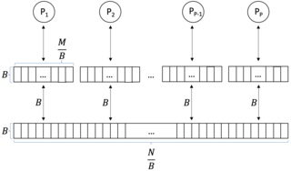
In computer science, a parallel external memory (PEM) model is a cache-aware, external-memory abstract machine. It is the parallel-computing analogy to the single-processor external memory (EM) model. In a similar way, it is the cache-aware analogy to the parallel random-access machine (PRAM). The PEM model consists of a number of processors, together with their respective private caches and a shared main memory.
References
- 1 2 3 4 Neubert, Karl-Dietrich (February 1998). "The Flashsort1 Algorithm". Dr. Dobb's Journal. 23 (2): 123–125, 131. Retrieved 2007-11-06.
- 1 2 Neubert, Karl-Dietrich (1998). "The FlashSort Algorithm" . Retrieved 2007-11-06.
- ↑ Xiao, Li; Zhang, Xiaodong; Kubricht, Stefan A. (2000). "Improving Memory Performance of Sorting Algorithms: Cache-Effective Quicksort". ACM Journal of Experimental Algorithmics. 5. CiteSeerX 10.1.1.43.736 . doi:10.1145/351827.384245. Archived from the original on 2007-11-02. Retrieved 2007-11-06.