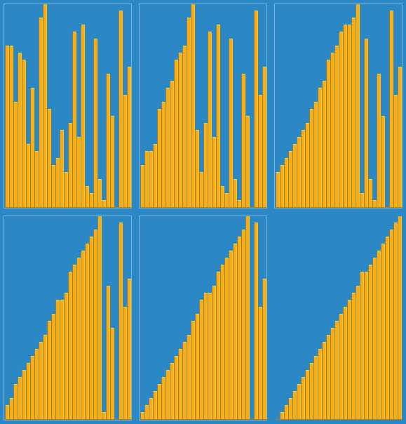
In computer science and information theory, a Huffman code is a particular type of optimal prefix code that is commonly used for lossless data compression. The process of finding or using such a code is Huffman coding, an algorithm developed by David A. Huffman while he was a Sc.D. student at MIT, and published in the 1952 paper "A Method for the Construction of Minimum-Redundancy Codes".

Insertion sort is a simple sorting algorithm that builds the final sorted array (or list) one item at a time by comparisons. It is much less efficient on large lists than more advanced algorithms such as quicksort, heapsort, or merge sort. However, insertion sort provides several advantages:
In computer science, radix sort is a non-comparative sorting algorithm. It avoids comparison by creating and distributing elements into buckets according to their radix. For elements with more than one significant digit, this bucketing process is repeated for each digit, while preserving the ordering of the prior step, until all digits have been considered. For this reason, radix sort has also been called bucket sort and digital sort.
In computer science, selection sort is an in-place comparison sorting algorithm. It has an O(n2) time complexity, which makes it inefficient on large lists, and generally performs worse than the similar insertion sort. Selection sort is noted for its simplicity and has performance advantages over more complicated algorithms in certain situations, particularly where auxiliary memory is limited.
The subset sum problem (SSP) is a decision problem in computer science. In its most general formulation, there is a multiset of integers and a target-sum , and the question is to decide whether any subset of the integers sum to precisely . The problem is known to be NP-complete. Moreover, some restricted variants of it are NP-complete too, for example:

Bucket sort, or bin sort, is a sorting algorithm that works by distributing the elements of an array into a number of buckets. Each bucket is then sorted individually, either using a different sorting algorithm, or by recursively applying the bucket sorting algorithm. It is a distribution sort, a generalization of pigeonhole sort that allows multiple keys per bucket, and is a cousin of radix sort in the most-to-least significant digit flavor. Bucket sort can be implemented with comparisons and therefore can also be considered a comparison sort algorithm. The computational complexity depends on the algorithm used to sort each bucket, the number of buckets to use, and whether the input is uniformly distributed.
In computer science, counting sort is an algorithm for sorting a collection of objects according to keys that are small positive integers; that is, it is an integer sorting algorithm. It operates by counting the number of objects that possess distinct key values, and applying prefix sum on those counts to determine the positions of each key value in the output sequence. Its running time is linear in the number of items and the difference between the maximum key value and the minimum key value, so it is only suitable for direct use in situations where the variation in keys is not significantly greater than the number of items. It is often used as a subroutine in radix sort, another sorting algorithm, which can handle larger keys more efficiently.
In computer science, bogosort is a sorting algorithm based on the generate and test paradigm. The function successively generates permutations of its input until it finds one that is sorted. It is not considered useful for sorting, but may be used for educational purposes, to contrast it with more efficient algorithms.
The Cooley–Tukey algorithm, named after J. W. Cooley and John Tukey, is the most common fast Fourier transform (FFT) algorithm. It re-expresses the discrete Fourier transform (DFT) of an arbitrary composite size in terms of N1 smaller DFTs of sizes N2, recursively, to reduce the computation time to O(N log N) for highly composite N (smooth numbers). Because of the algorithm's importance, specific variants and implementation styles have become known by their own names, as described below.
The Luhn algorithm or Luhn formula, also known as the "modulus 10" or "mod 10" algorithm, named after its creator, IBM scientist Hans Peter Luhn, is a simple check digit formula used to validate a variety of identification numbers. It is described in U.S. Patent No. 2,950,048, granted on August 23, 1960.

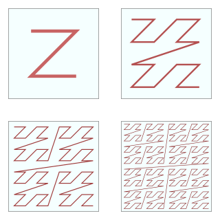
In mathematical analysis and computer science, functions which are Z-order, Lebesgue curve, Morton space-filling curve, Morton order or Morton code map multidimensional data to one dimension while preserving locality of the data points. It is named in France after Henri Lebesgue, who studied it in 1904, and named in the United States after Guy Macdonald Morton, who first applied the order to file sequencing in 1966. The z-value of a point in multidimensions is simply calculated by interleaving the binary representations of its coordinate values. Once the data are sorted into this ordering, any one-dimensional data structure can be used, such as simple one dimensional arrays, binary search trees, B-trees, skip lists or hash tables. The resulting ordering can equivalently be described as the order one would get from a depth-first traversal of a quadtree or octree.
The Hungarian method is a combinatorial optimization algorithm that solves the assignment problem in polynomial time and which anticipated later primal–dual methods. It was developed and published in 1955 by Harold Kuhn, who gave it the name "Hungarian method" because the algorithm was largely based on the earlier works of two Hungarian mathematicians, Dénes Kőnig and Jenő Egerváry. However, in 2006 it was discovered that Carl Gustav Jacobi had solved the assignment problem in the 19th century, and the solution had been published posthumously in 1890 in Latin.

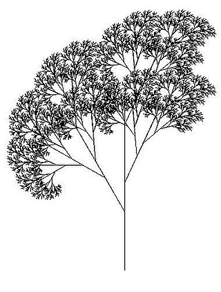
In computer science, recursion is a method of solving a computational problem where the solution depends on solutions to smaller instances of the same problem. Recursion solves such recursive problems by using functions that call themselves from within their own code. The approach can be applied to many types of problems, and recursion is one of the central ideas of computer science.
The power of recursion evidently lies in the possibility of defining an infinite set of objects by a finite statement. In the same manner, an infinite number of computations can be described by a finite recursive program, even if this program contains no explicit repetitions.
In numerical analysis and linear algebra, lower–upper (LU) decomposition or factorization factors a matrix as the product of a lower triangular matrix and an upper triangular matrix. The product sometimes includes a permutation matrix as well. LU decomposition can be viewed as the matrix form of Gaussian elimination. Computers usually solve square systems of linear equations using LU decomposition, and it is also a key step when inverting a matrix or computing the determinant of a matrix. The LU decomposition was introduced by the Polish astronomer Tadeusz Banachiewicz in 1938. To quote: "It appears that Gauss and Doolittle applied the method [of elimination] only to symmetric equations. More recent authors, for example, Aitken, Banachiewicz, Dwyer, and Crout … have emphasized the use of the method, or variations of it, in connection with non-symmetric problems … Banachiewicz … saw the point … that the basic problem is really one of matrix factorization, or “decomposition” as he called it." It is also sometimes referred to as LR decomposition.
The Luhn mod N algorithm is an extension to the Luhn algorithm that allows it to work with sequences of values in any even-numbered base. This can be useful when a check digit is required to validate an identification string composed of letters, a combination of letters and digits or any arbitrary set of N characters where N is divisible by 2.
In-place matrix transposition, also called in-situ matrix transposition, is the problem of transposing an N×M matrix in-place in computer memory, ideally with O(1) (bounded) additional storage, or at most with additional storage much less than NM. Typically, the matrix is assumed to be stored in row-major or column-major order.
In computer science, integer sorting is the algorithmic problem of sorting a collection of data values by integer keys. Algorithms designed for integer sorting may also often be applied to sorting problems in which the keys are floating point numbers, rational numbers, or text strings. The ability to perform integer arithmetic on the keys allows integer sorting algorithms to be faster than comparison sorting algorithms in many cases, depending on the details of which operations are allowed in the model of computing and how large the integers to be sorted are.

In computer science, sorting is the problem of sorting pairs of numbers by their sums. Applications of the problem include transit fare minimisation, VLSI design, and sparse polynomial multiplication. As with comparison sorting and integer sorting more generally, algorithms for this problem can be based only on comparisons of these sums, or on other operations that work only when the inputs are small integers.

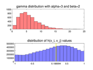
In statistics, the medcouple is a robust statistic that measures the skewness of a univariate distribution. It is defined as a scaled median difference between the left and right half of a distribution. Its robustness makes it suitable for identifying outliers in adjusted boxplots. Ordinary box plots do not fare well with skew distributions, since they label the longer unsymmetrical tails as outliers. Using the medcouple, the whiskers of a boxplot can be adjusted for skew distributions and thus have a more accurate identification of outliers for non-symmetrical distributions.
Interpolation sort is a sorting algorithm that is a kind of bucket sort. It uses an interpolation formula to assign data to the bucket. A general interpolation formula is:


