This is a glossary of graph theory. Graph theory is the study of graphs, systems of nodes or vertices connected in pairs by lines or edges.

In graph theory, graph coloring is a special case of graph labeling; it is an assignment of labels traditionally called "colors" to elements of a graph subject to certain constraints. In its simplest form, it is a way of coloring the vertices of a graph such that no two adjacent vertices are of the same color; this is called a vertex coloring. Similarly, an edge coloring assigns a color to each edge so that no two adjacent edges are of the same color, and a face coloring of a planar graph assigns a color to each face or region so that no two faces that share a boundary have the same color.

In graph theory, a perfect graph is a graph in which the chromatic number equals the size of the maximum clique, both in the graph itself and in every induced subgraph. In all graphs, the chromatic number is greater than or equal to the size of the maximum clique, but they can be far apart. A graph is perfect when these numbers are equal, and remain equal after the deletion of arbitrary subsets of vertices.

In graph theory, the perfect graph theorem of László Lovász states that an undirected graph is perfect if and only if its complement graph is also perfect. This result had been conjectured by Berge, and it is sometimes called the weak perfect graph theorem to distinguish it from the strong perfect graph theorem characterizing perfect graphs by their forbidden induced subgraphs.

In graph theory, a critical graph is an undirected graph all of whose proper subgraphs have smaller chromatic number. In such a graph, every vertex or edge is a critical element, in the sense that its deletion would decrease the number of colors needed in a graph coloring of the given graph. The decrease in the number of colors cannot be by more than one.

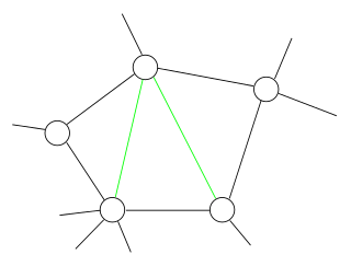
In graph theory, a proper edge coloring of a graph is an assignment of "colors" to the edges of the graph so that no two incident edges have the same color. For example, the figure to the right shows an edge coloring of a graph by the colors red, blue, and green. Edge colorings are one of several different types of graph coloring. The edge-coloring problem asks whether it is possible to color the edges of a given graph using at most k different colors, for a given value of k, or with the fewest possible colors. The minimum required number of colors for the edges of a given graph is called the chromatic index of the graph. For example, the edges of the graph in the illustration can be colored by three colors but cannot be colored by two colors, so the graph shown has chromatic index three.
In graph theory, a branch of mathematics, list coloring is a type of graph coloring where each vertex can be restricted to a list of allowed colors. It was first studied in the 1970s in independent papers by Vizing and by Erdős, Rubin, and Taylor.
In the mathematical area of graph theory, a chordal graph is one in which all cycles of four or more vertices have a chord, which is an edge that is not part of the cycle but connects two vertices of the cycle. Equivalently, every induced cycle in the graph should have exactly three vertices. The chordal graphs may also be characterized as the graphs that have perfect elimination orderings, as the graphs in which each minimal separator is a clique, and as the intersection graphs of subtrees of a tree. They are sometimes also called rigid circuit graphs or triangulated graphs: a chordal completion of a graph is typically called a triangulation of that graph.
In graph theory, a cograph, or complement-reducible graph, or P4-free graph, is a graph that can be generated from the single-vertex graph K1 by complementation and disjoint union. That is, the family of cographs is the smallest class of graphs that includes K1 and is closed under complementation and disjoint union.

In graph theory, the Grundy number or Grundy chromatic number of an undirected graph is the maximum number of colors that can be used by a greedy coloring strategy that considers the vertices of the graph in sequence and assigns each vertex its first available color, using a vertex ordering chosen to use as many colors as possible. Grundy numbers are named after P. M. Grundy, who studied an analogous concept for directed graphs in 1939. The undirected version was introduced by Christen & Selkow (1979).

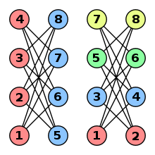
In the mathematical area of graph theory, Kőnig's theorem, proved by Dénes Kőnig, describes an equivalence between the maximum matching problem and the minimum vertex cover problem in bipartite graphs. It was discovered independently, also in 1931, by Jenő Egerváry in the more general case of weighted graphs.
In graph theory, a clique cover or partition into cliques of a given undirected graph is a partition of the vertices into cliques, subsets of vertices within which every two vertices are adjacent. A minimum clique cover is a clique cover that uses as few cliques as possible. The minimum k for which a clique cover exists is called the clique cover number of the given graph.
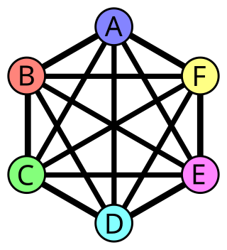
In graph theory, Brooks' theorem states a relationship between the maximum degree of a graph and its chromatic number. According to the theorem, in a connected graph in which every vertex has at most Δ neighbors, the vertices can be colored with only Δ colors, except for two cases, complete graphs and cycle graphs of odd length, which require Δ + 1 colors.
In graph theory, a perfectly orderable graph is a graph whose vertices can be ordered in such a way that a greedy coloring algorithm with that ordering optimally colors every induced subgraph of the given graph. Perfectly orderable graphs form a special case of the perfect graphs, and they include the chordal graphs, comparability graphs, and distance-hereditary graphs. However, testing whether a graph is perfectly orderable is NP-complete.
In graph theory, an area of mathematics, an equitable coloring is an assignment of colors to the vertices of an undirected graph, in such a way that
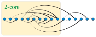
In graph theory, a k-degenerate graph is an undirected graph in which every subgraph has a vertex of degree at most k: that is, some vertex in the subgraph touches k or fewer of the subgraph's edges. The degeneracy of a graph is the smallest value of k for which it is k-degenerate. The degeneracy of a graph is a measure of how sparse it is, and is within a constant factor of other sparsity measures such as the arboricity of a graph.
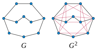
In graph theory, a branch of mathematics, the kth powerGk of an undirected graph G is another graph that has the same set of vertices, but in which two vertices are adjacent when their distance in G is at most k. Powers of graphs are referred to using terminology similar to that of exponentiation of numbers: G2 is called the square of G, G3 is called the cube of G, etc.

In graph theory, a subfield of mathematics, a well-colored graph is an undirected graph for which greedy coloring uses the same number of colors regardless of the order in which colors are chosen for its vertices. That is, for these graphs, the chromatic number and Grundy number are equal.

In the mathematics of graph coloring, Cereceda’s conjecture is an unsolved problem on the distance between pairs of colorings of sparse graphs. It states that, for two different colorings of a graph of degeneracy d, both using at most d + 2 colors, it should be possible to reconfigure one coloring into the other by changing the color of one vertex at a time, using a number of steps that is quadratic in the size of the graph. The conjecture is named after Luis Cereceda, who formulated it in his 2007 doctoral dissertation.
The Earth–Moon problem is an unsolved problem on graph coloring in mathematics. It is an extension of the planar map coloring problem, and was posed by Gerhard Ringel in 1959. In mathematical terms, it seeks the chromatic number of biplanar graphs. It is known that this number is at least 9 and at most 12.