Implicit curve

Last updated
Cassini ovals:
(1) a=1.1, c=1 (above),
(2) a=c=1 (middle),
(3) a=1, c=1.05 (below) Impl-c-cass-123.svg
Cassini ovals:
(1) a=1.1, c=1 (above),
(2) a=c=1 (middle),
(3) a=1, c=1.05 (below)
Implicit curve:
sin
[?]
(
x
+
y
)
-
cos
[?]
(
x
y
)
+
1
=
0
{\displaystyle \sin(x+y)-\cos(xy)+1=0} Ic-raster13-s.svg
Implicit curve:
Implicit curve
sin
[?]
(
x
+
y
)
-
cos
[?]
(
x
y
)
+
1
=
0
{\displaystyle \sin(x+y)-\cos(xy)+1=0}
as level curves of the surface
z
=
sin
[?]
(
x
+
y
)
-
cos
[?]
(
x
y
)
+
1
{\displaystyle z=\sin(x+y)-\cos(xy)+1} Fl-sin-cos-nivk-s.svg
Implicit curve as level curves of the surface

In mathematics, an implicit curve is a plane curve defined by an implicit equation relating two coordinate variables, commonly x and y. For example, the unit circle is defined by the implicit equation . In general, every implicit curve is defined by an equation of the form

Contents

for some function F of two variables. Hence an implicit curve can be considered as the set of zeros of a function of two variables. Implicit means that the equation is not expressed as a solution for either x in terms of y or vice versa.

If is a polynomial in two variables, the corresponding curve is called an algebraic curve , and specific methods are available for studying it.

Plane curves can be represented in Cartesian coordinates (x, y coordinates) by any of three methods, one of which is the implicit equation given above. The graph of a function is usually described by an equation in which the functional form is explicitly stated; this is called an explicit representation. The third essential description of a curve is the parametric one, where the x- and y-coordinates of curve points are represented by two functions x(t), y(t) both of whose functional forms are explicitly stated, and which are dependent on a common parameter

Examples of implicit curves include:

  1. a line:
  2. a circle:
  3. the semicubical parabola:
  4. Cassini ovals (see diagram),
  5. (see diagram).

The first four examples are algebraic curves, but the last one is not algebraic. The first three examples possess simple parametric representations, which is not true for the fourth and fifth examples. The fifth example shows the possibly complicated geometric structure of an implicit curve.

The implicit function theorem describes conditions under which an equation can be solved implicitly for x and/or y – that is, under which one can validly write or . This theorem is the key for the computation of essential geometric features of the curve: tangents, normals, and curvature. In practice implicit curves have an essential drawback: their visualization is difficult. But there are computer programs enabling one to display an implicit curve. Special properties of implicit curves make them essential tools in geometry and computer graphics.

An implicit curve with an equation can be considered as the level curve of level 0 of the surface (see third diagram).

Slope and curvature

In general, implicit curves fail the vertical line test (meaning that some values of x are associated with more than one value of y) and so are not necessarily graphs of functions. However, the implicit function theorem gives conditions under which an implicit curve locally is given by the graph of a function (so in particular it has no self-intersections). If the defining relations are sufficiently smooth then, in such regions, implicit curves have well defined slopes, tangent lines, normal vectors, and curvature.

There are several possible ways to compute these quantities for a given implicit curve. One method is to use implicit differentiation to compute the derivatives of y with respect to x. Alternatively, for a curve defined by the implicit equation , one can express these formulas directly in terms of the partial derivatives of . In what follows, the partial derivatives are denoted (for the derivative with respect to x), , (for the second partial with respect to x), (for the mixed second partial),

Tangent and normal vector

A curve point is regular if the first partial derivatives and are not both equal to 0.

The equation of the tangent line at a regular point is

so the slope of the tangent line, and hence the slope of the curve at that point, is

If at the curve is vertical at that point, while if both and at that point then the curve is not differentiable there, but instead is a singular point – either a cusp or a point where the curve intersects itself.

A normal vector to the curve at the point is given by

(here written as a row vector).

Curvature

For readability of the formulas, the arguments are omitted. The curvature at a regular point is given by the formula

. [1]

Derivation of the formulas

The implicit function theorem guarantees within a neighborhood of a point the existence of a function such that . By the chain rule, the derivatives of function are

and

(where the arguments on the right side of the second formula are omitted for ease of reading).

Inserting the derivatives of function into the formulas for a tangent and curvature of the graph of the explicit equation yields

(tangent)
(curvature).

Advantage and disadvantage of implicit curves

Disadvantage

The essential disadvantage of an implicit curve is the lack of an easy possibility to calculate single points which is necessary for visualization of an implicit curve (see next section).

Advantages

  1. Implicit representations facilitate the computation of intersection points: If one curve is represented implicitly and the other parametrically the computation of intersection points needs only a simple (1-dimensional) Newton iteration, which is contrary to the cases implicit-implicit and parametric-parametric (see Intersection).
  2. An implicit representation gives the possibility of separating points not on the curve by the sign of . This may be helpful for example applying the false position method instead of a Newton iteration.
  3. It is easy to generate curves which are almost geometrically similar to the given implicit curve by just adding a small number: (see section #Smooth approximations).

Applications of implicit curves

Smooth approximation of a convex polygon Ic-approx-haus.svg
Smooth approximation of a convex polygon
Smooth approximation of 1)one half of a circle, 2) an intersection of two circles Ic-approx-kg-k2.svg
Smooth approximation of 1)one half of a circle, 2) an intersection of two circles

Within mathematics implicit curves play a prominent role as algebraic curves. In addition, implicit curves are used for designing curves of desired geometrical shapes. Here are two examples.

Smooth approximations

Convex polygons

A smooth approximation of a convex polygon can be achieved in the following way: Let be the equations of the lines containing the edges of the polygon such that for an inner point of the polygon is positive. Then a subset of the implicit curve

with suitable small parameter is a smooth (differentiable) approximation of the polygon. For example, the curves

for

contain smooth approximations of a polygon with 5 edges (see diagram).

Pairs of lines

In case of two lines

one gets

a pencil of parallel lines, if the given lines are parallel or
the pencil of hyperbolas, which have the given lines as asymptotes.

For example, the product of the coordinate axes variables yields the pencil of hyperbolas , which have the coordinate axes as asymptotes.

Others

If one starts with simple implicit curves other than lines (circles, parabolas,...) one gets a wide range of interesting new curves. For example,

(product of a circle and the x-axis) yields smooth approximations of one half of a circle (see picture), and

(product of two circles) yields smooth approximations of the intersection of two circles (see diagram).

Blending curves

Blending curve (red) of two circles Parab-f-spline-2k2g.svg
Blending curve (red) of two circles

In CAD one uses implicit curves for the generation of blending curves, [2] [3] which are special curves establishing a smooth transition between two given curves. For example,

generates blending curves between the two circles

The method guarantees the continuity of the tangents and curvatures at the points of contact (see diagram). The two lines

determine the points of contact at the circles. Parameter is a design parameter. In the diagram, .

Equipotential curves of two point charges

Equipotential curves of two point charges at the blue points Impl-ku-lad2.svg
Equipotential curves of two point charges at the blue points

Equipotential curves of two equal point charges at the points can be represented by the equation

The curves are similar to Cassini ovals, but they are not such curves.

Visualization of an implicit curve

To visualize an implicit curve one usually determines a polygon on the curve and displays the polygon. For a parametric curve this is an easy task: One just computes the points of a sequence of parametric values. For an implicit curve one has to solve two subproblems:

  1. determination of a first curve point to a given starting point in the vicinity of the curve,
  2. determination of a curve point starting from a known curve point.

In both cases it is reasonable to assume . In practice this assumption is violated at single isolated points only.

Point algorithm

For the solution of both tasks mentioned above it is essential to have a computer program (which we will call ), which, when given a point near an implicit curve, finds a point that is exactly on the curve, up to the accuracy of computation:

(P1) for the start point is
(P2)repeat
(Newton step for function )
(P3)until the distance between the points is small enough.
(P4) is the curve point near the start point .

Tracing algorithm

to the tracing algorithm: starting points are green Impl-punkt-algor-s.svg
to the tracing algorithm: starting points are green

In order to generate a nearly equally spaced polygon on the implicit curve one chooses a step length and

(T1) chooses a suitable starting point in the vicinity of the curve
(T2) determines a first curve point using program
(T3) determines the tangent (see above), chooses a starting point on the tangent using step length (see diagram) and determines a second curve point using program .

Because the algorithm traces the implicit curve it is called a tracing algorithm. The algorithm traces only connected parts of the curve. If the implicit curve consists of several parts it has to be started several times with suitable starting points.

Example: An illustration of the raster algorithm applied to the implicit curve
F
(
x
,
y
)
=
(
3
x
2
-
y
2
)
2
y
2
-
(
x
2
+
y
2
)
4
=
0
{\displaystyle F(x,y)=(3x^{2}-y^{2})^{2}y^{2}-(x^{2}+y^{2})^{4}=0}
. The curve (red) is what the algorithm is trying to draw. The raster points (black) are used as starting points to find the closest points on the curve (red circles). The spacing between each raster point is exaggerated to show the individual curve points; to more accurately trace the curve, more raster points would be used. Icraster-blume.svg
Example: An illustration of the raster algorithm applied to the implicit curve . The curve (red) is what the algorithm is trying to draw. The raster points (black) are used as starting points to find the closest points on the curve (red circles). The spacing between each raster point is exaggerated to show the individual curve points; to more accurately trace the curve, more raster points would be used.

Raster algorithm

If the implicit curve consists of several or even unknown parts, it may be better to use a rasterisation algorithm. Instead of exactly following the curve, a raster algorithm covers the entire curve in so many points that they blend together and look like the curve.

(R1) Generate a net of points (raster) on the area of interest of the x-y-plane.
(R2) For every point in the raster, run the point algorithm starting from P, then mark its output.

If the net is dense enough, the result approximates the connected parts of the implicit curve. If for further applications polygons on the curves are needed one can trace parts of interest by the tracing algorithm.

Implicit space curves

Any space curve which is defined by two equations

is called an implicit space curve.

A curve point is called regular if the cross product of the gradients and is not at this point:

otherwise it is called singular. Vector is a tangent vector of the curve at point

Intersection curve between a sphere and a cylinder Is-spherecyl5-s.svg
Intersection curve between a sphere and a cylinder

Examples:

is a line.

is a plane section of a sphere, hence a circle.

is an ellipse (plane section of a cylinder).

is the intersection curve between a sphere and a cylinder.

For the computation of curve points and the visualization of an implicit space curve see Intersection.

See also

Related Research Articles

<span class="mw-page-title-main">Ellipse</span> Plane curve: conic section

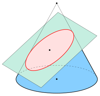
In mathematics, an ellipse is a plane curve surrounding two focal points, such that for all points on the curve, the sum of the two distances to the focal points is a constant. It generalizes a circle, which is the special type of ellipse in which the two focal points are the same. The elongation of an ellipse is measured by its eccentricity , a number ranging from to .

<span class="mw-page-title-main">Parabola</span> Plane curve: conic section

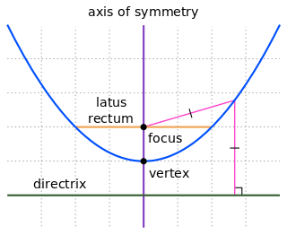
In mathematics, a parabola is a plane curve which is mirror-symmetrical and is approximately U-shaped. It fits several superficially different mathematical descriptions, which can all be proved to define exactly the same curves.

<span class="mw-page-title-main">Tangent</span> In mathematics, straight line touching a plane curve without crossing it

In geometry, the tangent line (or simply tangent) to a plane curve at a given point is, intuitively, the straight line that "just touches" the curve at that point. Leibniz defined it as the line through a pair of infinitely close points on the curve. More precisely, a straight line is tangent to the curve y = f(x) at a point x = c if the line passes through the point (c, f(c)) on the curve and has slope f'(c), where f' is the derivative of f. A similar definition applies to space curves and curves in n-dimensional Euclidean space.

<span class="mw-page-title-main">Curvature</span> Mathematical measure of how much a curve or surface deviates from flatness

In mathematics, curvature is any of several strongly related concepts in geometry that intuitively measure the amount by which a curve deviates from being a straight line or by which a surface deviates from being a plane. If a curve or surface is contained in a larger space, curvature can be defined extrinsically relative to the ambient space. Curvature of Riemannian manifolds of dimension at least two can be defined intrinsically without reference to a larger space.

<span class="mw-page-title-main">Winding number</span> Number of times a curve wraps around a point in the plane

In mathematics, the winding number or winding index of a closed curve in the plane around a given point is an integer representing the total number of times that the curve travels counterclockwise around the point, i.e., the curve's number of turns. For certain open plane curves, the number of turns may be a non-integer. The winding number depends on the orientation of the curve, and it is negative if the curve travels around the point clockwise.

<span class="mw-page-title-main">Normal (geometry)</span> Line or vector perpendicular to a curve or a surface

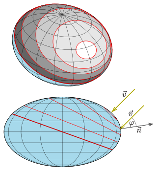
In geometry, a normal is an object that is perpendicular to a given object. For example, the normal line to a plane curve at a given point is the line perpendicular to the tangent line to the curve at the point.

<span class="mw-page-title-main">Algebraic curve</span> Curve defined as zeros of polynomials

In mathematics, an affine algebraic plane curve is the zero set of a polynomial in two variables. A projective algebraic plane curve is the zero set in a projective plane of a homogeneous polynomial in three variables. An affine algebraic plane curve can be completed in a projective algebraic plane curve by homogenizing its defining polynomial. Conversely, a projective algebraic plane curve of homogeneous equation h(x, y, t) = 0 can be restricted to the affine algebraic plane curve of equation h(x, y, 1) = 0. These two operations are each inverse to the other; therefore, the phrase algebraic plane curve is often used without specifying explicitly whether it is the affine or the projective case that is considered.

<span class="mw-page-title-main">Parametric equation</span> Representation of a curve by a function of a parameter

In mathematics, a parametric equation defines a group of quantities as functions of one or more independent variables called parameters. Parametric equations are commonly used to express the coordinates of the points that make up a geometric object such as a curve or surface, called a parametric curve and parametric surface, respectively. In such cases, the equations are collectively called a parametric representation, or parametric system, or parameterization of the object.

<span class="mw-page-title-main">Cardioid</span> Type of plane curve

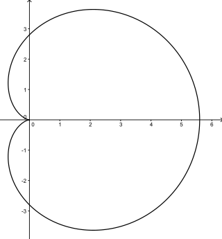
In geometry, a cardioid is a plane curve traced by a point on the perimeter of a circle that is rolling around a fixed circle of the same radius. It can also be defined as an epicycloid having a single cusp. It is also a type of sinusoidal spiral, and an inverse curve of the parabola with the focus as the center of inversion. A cardioid can also be defined as the set of points of reflections of a fixed point on a circle through all tangents to the circle.

<span class="mw-page-title-main">Dupin cyclide</span> Geometric inversion of a torus, cylinder or double cone

In mathematics, a Dupin cyclide or cyclide of Dupin is any geometric inversion of a standard torus, cylinder or double cone. In particular, these latter are themselves examples of Dupin cyclides. They were discovered c. 1802 by Charles Dupin, while he was still a student at the École polytechnique following Gaspard Monge's lectures. The key property of a Dupin cyclide is that it is a channel surface in two different ways. This property means that Dupin cyclides are natural objects in Lie sphere geometry.

<span class="mw-page-title-main">Parallel curve</span>

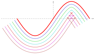
A parallel of a curve is the envelope of a family of congruent circles centered on the curve. It generalises the concept of parallel (straight) lines. It can also be defined as a curve whose points are at a constant normal distance from a given curve. These two definitions are not entirely equivalent as the latter assumes smoothness, whereas the former does not.

<span class="mw-page-title-main">Implicit surface</span> Surface in 3D space defined by an implicit function of three variables

In mathematics, an implicit surface is a surface in Euclidean space defined by an equation

<span class="mw-page-title-main">Osculating circle</span> Circle of immediate corresponding curvature of a curve at a point

An osculating circle is a circle that best approximates the curvature of a curve at a specific point. It is tangent to the curve at that point and has the same curvature as the curve at that point. The osculating circle provides a way to understand the local behavior of a curve and is commonly used in differential geometry and calculus.

<span class="mw-page-title-main">Dual curve</span> Curve in the dual projective plane made from all lines tangent to a given curve

In projective geometry, a dual curve of a given plane curve C is a curve in the dual projective plane consisting of the set of lines tangent to C. There is a map from a curve to its dual, sending each point to the point dual to its tangent line. If C is algebraic then so is its dual and the degree of the dual is known as the class of the original curve. The equation of the dual of C, given in line coordinates, is known as the tangential equation of C. Duality is an involution: the dual of the dual of C is the original curve C.

A parametric surface is a surface in the Euclidean space which is defined by a parametric equation with two parameters . Parametric representation is a very general way to specify a surface, as well as implicit representation. Surfaces that occur in two of the main theorems of vector calculus, Stokes' theorem and the divergence theorem, are frequently given in a parametric form. The curvature and arc length of curves on the surface, surface area, differential geometric invariants such as the first and second fundamental forms, Gaussian, mean, and principal curvatures can all be computed from a given parametrization.

<span class="mw-page-title-main">Surface (mathematics)</span> Mathematical idealization of the surface of a body

In mathematics, a surface is a mathematical model of the common concept of a surface. It is a generalization of a plane, but, unlike a plane, it may be curved; this is analogous to a curve generalizing a straight line.

<span class="mw-page-title-main">Differential geometry of surfaces</span> The mathematics of smooth surfaces

In mathematics, the differential geometry of surfaces deals with the differential geometry of smooth surfaces with various additional structures, most often, a Riemannian metric. Surfaces have been extensively studied from various perspectives: extrinsically, relating to their embedding in Euclidean space and intrinsically, reflecting their properties determined solely by the distance within the surface as measured along curves on the surface. One of the fundamental concepts investigated is the Gaussian curvature, first studied in depth by Carl Friedrich Gauss, who showed that curvature was an intrinsic property of a surface, independent of its isometric embedding in Euclidean space.

<span class="mw-page-title-main">Isophote</span> Curve on an illuminated surface through points of equal brightness

In geometry, an isophote is a curve on an illuminated surface that connects points of equal brightness. One supposes that the illumination is done by parallel light and the brightness b is measured by the following scalar product:

<span class="mw-page-title-main">Intersection (geometry)</span> Shape formed from points common to other shapes

In geometry, an intersection is a point, line, or curve common to two or more objects. The simplest case in Euclidean geometry is the line–line intersection between two distinct lines, which either is one point or does not exist. Other types of geometric intersection include:

<span class="mw-page-title-main">Intersection curve</span> Curve that is common to two geometric objects

In geometry, an intersection curve is a curve that is common to two geometric objects. In the simplest case, the intersection of two non-parallel planes in Euclidean 3-space is a line. In general, an intersection curve consists of the common points of two transversally intersecting surfaces, meaning that at any common point the surface normals are not parallel. This restriction excludes cases where the surfaces are touching or have surface parts in common.

References

  1. Goldman, R. (2005). "Curvature formulas for implicit curves and surfaces". Computer Aided Geometric Design. 22 (7): 632–658. CiteSeerX   10.1.1.413.3008 . doi:10.1016/j.cagd.2005.06.005.
  2. C. Hoffmann & J. Hopcroft: The potential method for blending surfaces and corners in G. Farin (Ed) Geometric-Modeling, SIAM, Philadelphia, pp. 347-365
  3. E. Hartmann: Blending of implicit surfaces with functional splines, CAD,Butterworth-Heinemann, Volume 22 (8), 1990, p. 500-507
  4. G. Taubin: Distance Approximations for Rastering Implicit Curves. ACM Transactions on Graphics, Vol. 13, No. 1, 1994.