Score (statistics)

Last updated July 13, 2023

In statistics, the score (or informant^[1]) is the gradient of the log-likelihood function with respect to the parameter vector. Evaluated at a particular point of the parameter vector, the score indicates the steepness of the log-likelihood function and thereby the sensitivity to infinitesimal changes to the parameter values. If the log-likelihood function is continuous over the parameter space, the score will vanish at a local maximum or minimum; this fact is used in maximum likelihood estimation to find the parameter values that maximize the likelihood function.

Since the score is a function of the observations that are subject to sampling error, it lends itself to a test statistic known as score test in which the parameter is held at a particular value. Further, the ratio of two likelihood functions evaluated at two distinct parameter values can be understood as a definite integral of the score function.^[2]

Definition

The score is the gradient (the vector of partial derivatives) of $\log {\mathcal {L}}(\theta )$ , the natural logarithm of the likelihood function, with respect to an m-dimensional parameter vector $\theta$ .

s(\theta )\equiv {\frac {\partial \log {\mathcal {L}}(\theta )}{\partial \theta }}

This differentiation yields a $(1\times m)$ row vector, and indicates the sensitivity of the likelihood (its derivative normalized by its value).

In older literature,^{[ citation needed ]} "linear score" may refer to the score with respect to infinitesimal translation of a given density. This convention arises from a time when the primary parameter of interest was the mean or median of a distribution. In this case, the likelihood of an observation is given by a density of the form ${\mathcal {L}}(\theta ;X)=f(X+\theta )$ . The "linear score" is then defined as

s_{\rm {linear}}={\frac {\partial }{\partial X}}\log f(X)

Properties

Mean

While the score is a function of $\theta$ , it also depends on the observations $\mathbf {x} =(x_{1},x_{2},\ldots x_{T})$ at which the likelihood function is evaluated, and in view of the random character of sampling one may take its expected value over the sample space. Under certain regularity conditions on the density functions of the random variables,^[3]^[4] the expected value of the score, evaluated at the true parameter value $\theta$ , is zero. To see this, rewrite the likelihood function ${\mathcal {L}}$ as a probability density function ${\mathcal {L}}(\theta ;x)=f(x;\theta )$ , and denote the sample space ${\mathcal {X}}$ . Then:

{\begin{aligned}\operatorname {E} (s\mid \theta )&=\int _{\mathcal {X}}f(x;\theta ){\frac {\partial }{\partial \theta }}\log {\mathcal {L}}(\theta ;x)\,dx\\[6pt]&=\int _{\mathcal {X}}f(x;\theta ){\frac {1}{f(x;\theta )}}{\frac {\partial f(x;\theta )}{\partial \theta }}\,dx=\int _{\mathcal {X}}{\frac {\partial f(x;\theta )}{\partial \theta }}\,dx\end{aligned}}

The assumed regularity conditions allow the interchange of derivative and integral (see Leibniz integral rule), hence the above expression may be rewritten as

{\frac {\partial }{\partial \theta }}\int _{\mathcal {X}}f(x;\theta )\,dx={\frac {\partial }{\partial \theta }}1=0.

It is worth restating the above result in words: the expected value of the score, at true parameter value $\theta$ is zero. Thus, if one were to repeatedly sample from some distribution, and repeatedly calculate the score, then the mean value of the scores would tend to zero asymptotically.

Variance

The variance of the score, $\operatorname {Var} (s(\theta ))=\operatorname {E} (s(\theta )s(\theta )^{\mathsf {T}})$ , can be derived from the above expression for the expected value.

{\begin{aligned}0&={\frac {\partial }{\partial \theta ^{\mathsf {T}}}}\operatorname {E} (s\mid \theta )\\[6pt]&={\frac {\partial }{\partial \theta ^{\mathsf {T}}}}\int _{\mathcal {X}}{\frac {\partial \log {\mathcal {L}}(\theta ;X)}{\partial \theta }}f(x;\theta )\,dx\\[6pt]&=\int _{\mathcal {X}}{\frac {\partial }{\partial \theta ^{\mathsf {T}}}}\left\{{\frac {\partial \log {\mathcal {L}}(\theta ;X)}{\partial \theta }}f(x;\theta )\right\}\,dx\\[6pt]&=\int _{\mathcal {X}}\left\{{\frac {\partial ^{2}\log {\mathcal {L}}(\theta ;X)}{\partial \theta \partial \theta ^{\mathsf {T}}}}f(x;\theta )+{\frac {\partial \log {\mathcal {L}}(\theta ;X)}{\partial \theta }}{\frac {\partial f(x;\theta )}{\partial \theta ^{\mathsf {T}}}}\right\}\,dx\\[6pt]&=\int _{\mathcal {X}}{\frac {\partial ^{2}\log {\mathcal {L}}(\theta ;X)}{\partial \theta \partial \theta ^{\mathsf {T}}}}f(x;\theta )\,dx+\int _{\mathcal {X}}{\frac {\partial \log {\mathcal {L}}(\theta ;X)}{\partial \theta }}{\frac {\partial f(x;\theta )}{\partial \theta ^{\mathsf {T}}}}\,dx\\[6pt]&=\int _{\mathcal {X}}{\frac {\partial ^{2}\log {\mathcal {L}}(\theta ;X)}{\partial \theta \partial \theta ^{\mathsf {T}}}}f(x;\theta )\,dx+\int _{\mathcal {X}}{\frac {\partial \log {\mathcal {L}}(\theta ;X)}{\partial \theta }}{\frac {\partial \log {\mathcal {L}}(\theta ;X)}{\partial \theta ^{\mathsf {T}}}}f(x;\theta )\,dx\\[6pt]&=\operatorname {E} \left({\frac {\partial ^{2}\log {\mathcal {L}}(\theta ;X)}{\partial \theta \partial \theta ^{\mathsf {T}}}}\right)+\operatorname {E} \left({\frac {\partial \log {\mathcal {L}}(\theta ;X)}{\partial \theta }}\left[{\frac {\partial \log {\mathcal {L}}(\theta ;X)}{\partial \theta }}\right]^{\mathsf {T}}\right)\end{aligned}}

Hence the variance of the score is equal to the negative expected value of the Hessian matrix of the log-likelihood.^[5]

\operatorname {E} (s(\theta )s(\theta )^{\mathsf {T}})=-\operatorname {E} \left({\frac {\partial ^{2}\log {\mathcal {L}}}{\partial \theta \partial \theta ^{\mathsf {T}}}}\right)

The latter is known as the Fisher information and is written ${\mathcal {I}}(\theta )$ . Note that the Fisher information is not a function of any particular observation, as the random variable $X$ has been averaged out. This concept of information is useful when comparing two methods of observation of some random process.

Examples

Bernoulli process

Consider observing the first n trials of a Bernoulli process, and seeing that A of them are successes and the remaining B are failures, where the probability of success is θ.

Then the likelihood ${\mathcal {L}}$ is

{\mathcal {L}}(\theta ;A,B)={\frac {(A+B)!}{A!B!}}\theta ^{A}(1-\theta )^{B},

so the score s is

s={\frac {1}{\mathcal {L}}}{\frac {\partial {\mathcal {L}}}{\partial \theta }}={\frac {A}{\theta }}-{\frac {B}{1-\theta }}.

We can now verify that the expectation of the score is zero. Noting that the expectation of A is nθ and the expectation of B is n(1 − θ) [recall that A and B are random variables], we can see that the expectation of s is

E(s)={\frac {n\theta }{\theta }}-{\frac {n(1-\theta )}{1-\theta }}=n-n=0.

We can also check the variance of $s$ . We know that A + B = n (so B = n − A) and the variance of A is nθ(1 − θ) so the variance of s is

{\begin{aligned}\operatorname {var} (s)&=\operatorname {var} \left({\frac {A}{\theta }}-{\frac {n-A}{1-\theta }}\right)=\operatorname {var} \left(A\left({\frac {1}{\theta }}+{\frac {1}{1-\theta }}\right)\right)\\&=\left({\frac {1}{\theta }}+{\frac {1}{1-\theta }}\right)^{2}\operatorname {var} (A)={\frac {n}{\theta (1-\theta )}}.\end{aligned}}

Binary outcome model

For models with binary outcomes (Y = 1 or 0), the model can be scored with the logarithm of predictions

S=Y\log(p)+(1-Y)(\log(1-p))

where p is the probability in the model to be estimated and S is the score.^[6]

Applications

Scoring algorithm

The scoring algorithm is an iterative method for numerically determining the maximum likelihood estimator.

Score test

Note that $s$ is a function of $\theta$ and the observation $\mathbf {x} =(x_{1},x_{2},\ldots x_{T})$ , so that, in general, it is not a statistic. However, in certain applications, such as the score test, the score is evaluated at a specific value of $\theta$ (such as a null-hypothesis value), in which case the result is a statistic. Intuitively, if the restricted estimator is near the maximum of the likelihood function, the score should not differ from zero by more than sampling error. In 1948, C. R. Rao first proved that the square of the score divided by the information matrix follows an asymptotic χ²-distribution under the null hypothesis.^[7]

Further note that the likelihood-ratio test is given by

-2\left[\log {\mathcal {L}}(\theta _{0})-\log {\mathcal {L}}({\hat {\theta }})\right]=2\int _{\theta _{0}}^{\hat {\theta }}{\frac {d\,\log {\mathcal {L}}(\theta )}{d\theta }}\,d\theta =2\int _{\theta _{0}}^{\hat {\theta }}s(\theta )\,d\theta

which means that the likelihood-ratio test can be understood as the area under the score function between $\theta _{0}$ and ${\hat {\theta }}$ .^[8]

Score matching (machine learning)

Score matching describes the process of applying machine learning algorithms (commonly neural networks) to approximate the score function $s_{\theta }\approx \nabla _{x}\log p(x)$ of an unknown distribution $\pi (x)$ from finite samples. The learned function $s_{\theta }$ can then be used in generative modeling to draw new samples from $\pi (x)$ .^[9]

It might seem confusing that the word score has been used for $\nabla _{x}\log p(x)$ , because it is not a likelihood function, neither it has a derivative with respect to the parameters. For more information about this definition, see the referenced paper. ^[10]

Notes

↑ Informant in Encyclopaedia of Maths
↑ Pickles, Andrew (1985). An Introduction to Likelihood Analysis. Norwich: W. H. Hutchins & Sons. pp. 24–29. ISBN 0-86094-190-6.
↑ Serfling, Robert J. (1980). Approximation Theorems of Mathematical Statistics . New York: John Wiley & Sons. p. 145. ISBN 0-471-02403-1.
↑ Greenberg, Edward; Webster, Charles E. Jr. (1983). Advanced Econometrics : A Bridge to the Literature. New York: John Wiley & Sons. p. 25. ISBN 0-471-09077-8.
↑ Sargan, Denis (1988). Lectures on Advanced Econometrics. Oxford: Basil Blackwell. pp. 16–18. ISBN 0-631-14956-2.
↑ Steyerberg, E. W.; Vickers, A. J.; Cook, N. R.; Gerds, T.; Gonen, M.; Obuchowski, N.; Pencina, M. J.; Kattan, M. W. (2010). "Assessing the performance of prediction models. A framework for traditional and novel measures". Epidemiology . 21 (1): 128–138. doi:10.1097/EDE.0b013e3181c30fb2. PMC 3575184 . PMID 20010215.
↑ Rao, C. Radhakrishna (1948). "Large sample tests of statistical hypotheses concerning several parameters with applications to problems of estimation". Mathematical Proceedings of the Cambridge Philosophical Society . 44 (1): 50–57. Bibcode:1948PCPS...44...50R. doi:10.1017/S0305004100023987. S2CID 122382660.
↑ Buse, A. (1982). "The Likelihood Ratio, Wald, and Lagrange Multiplier Tests: An Expository Note". The American Statistician . 36 (3a): 153–157. doi:10.1080/00031305.1982.10482817.
↑ Yang Song, Jascha Sohl-Dickstein, Diederik P. Kingma, Abhishek Kumar, Stefano Ermon, Ben Poole (2020). "Score-Based Generative Modeling through Stochastic Differential Equations". arXiv: 2011.13456 [cs.LG].{{cite arxiv}}: CS1 maint: uses authors parameter (link)
↑ https://www.jmlr.org/papers/volume6/hyvarinen05a/hyvarinen05a.pdf

Related Research Articles

The likelihood function is the joint probability of the observed data viewed as a function of the parameters of a statistical model.

In statistics, maximum likelihood estimation (MLE) is a method of estimating the parameters of an assumed probability distribution, given some observed data. This is achieved by maximizing a likelihood function so that, under the assumed statistical model, the observed data is most probable. The point in the parameter space that maximizes the likelihood function is called the maximum likelihood estimate. The logic of maximum likelihood is both intuitive and flexible, and as such the method has become a dominant means of statistical inference.

In probability theory and statistics, the beta distribution is a family of continuous probability distributions defined on the interval [0, 1] in terms of two positive parameters, denoted by alpha (α) and beta (β), that appear as exponents of the variable and its complement to 1, respectively, and control the shape of the distribution.

In mathematics, a Gaussian function, often simply referred to as a Gaussian, is a function of the base form

In probability theory and statistics, a Gaussian process is a stochastic process, such that every finite collection of those random variables has a multivariate normal distribution, i.e. every finite linear combination of them is normally distributed. The distribution of a Gaussian process is the joint distribution of all those random variables, and as such, it is a distribution over functions with a continuous domain, e.g. time or space.

In probability and statistics, an exponential family is a parametric set of probability distributions of a certain form, specified below. This special form is chosen for mathematical convenience, including the enabling of the user to calculate expectations, covariances using differentiation based on some useful algebraic properties, as well as for generality, as exponential families are in a sense very natural sets of distributions to consider. The term exponential class is sometimes used in place of "exponential family", or the older term Koopman–Darmois family. The terms "distribution" and "family" are often used loosely: specifically, an exponential family is a set of distributions, where the specific distribution varies with the parameter; however, a parametric family of distributions is often referred to as "a distribution", and the set of all exponential families is sometimes loosely referred to as "the" exponential family. They are distinct because they possess a variety of desirable properties, most importantly the existence of a sufficient statistic.

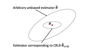
In estimation theory and statistics, the Cramér–Rao bound (CRB) relates to estimation of a deterministic parameter. The result is named in honor of Harald Cramér and C. R. Rao, but has also been derived independently by Maurice Fréchet, Georges Darmois, and by Alexander Aitken and Harold Silverstone. It states that the precision of any unbiased estimator is at most the Fisher information; or (equivalently) the inverse of the Fisher information is a lower bound on its variance.

In mathematical statistics, the Fisher information is a way of measuring the amount of information that an observable random variable X carries about an unknown parameter θ of a distribution that models X. Formally, it is the variance of the score, or the expected value of the observed information.

In mathematical statistics, the Kullback–Leibler divergence, denoted $, is a type of statistical distance: a measure of how one probability distribution P is different from a second, reference probability distribution Q . A simple interpretation of the KL divergence of P from Q is the expected excess surprise from using Q as a model when the actual distribution is P . While it is a distance, it is not a metric, the most familiar type of distance: it is not symmetric in the two distributions, and does not satisfy the triangle inequality. Instead, in terms of information geometry, it is a type of divergence, a generalization of squared distance, and for certain classes of distributions, it satisfies a generalized Pythagorean theorem.$

In statistics, the score test assesses constraints on statistical parameters based on the gradient of the likelihood function—known as the score—evaluated at the hypothesized parameter value under the null hypothesis. Intuitively, if the restricted estimator is near the maximum of the likelihood function, the score should not differ from zero by more than sampling error. While the finite sample distributions of score tests are generally unknown, they have an asymptotic χ²-distribution under the null hypothesis as first proved by C. R. Rao in 1948, a fact that can be used to determine statistical significance.

In decision theory and estimation theory, Stein's example is the observation that when three or more parameters are estimated simultaneously, there exist combined estimators more accurate on average than any method that handles the parameters separately. It is named after Charles Stein of Stanford University, who discovered the phenomenon in 1955.

In Bayesian probability, the Jeffreys prior, named after Sir Harold Jeffreys, is a non-informative prior distribution for a parameter space; its density function is proportional to the square root of the determinant of the Fisher information matrix:

In statistics, the delta method is a result concerning the approximate probability distribution for a function of an asymptotically normal statistical estimator from knowledge of the limiting variance of that estimator.

In statistics, M-estimators are a broad class of extremum estimators for which the objective function is a sample average. Both non-linear least squares and maximum likelihood estimation are special cases of M-estimators. The definition of M-estimators was motivated by robust statistics, which contributed new types of M-estimators. However, M-estimators are not inherently robust, as is clear from the fact that they include maximum likelihood estimators, which are in general not robust. The statistical procedure of evaluating an M-estimator on a data set is called M-estimation. 48 samples of robust M-estimators can be found in a recent review study.

In information theory and statistics, Kullback's inequality is a lower bound on the Kullback–Leibler divergence expressed in terms of the large deviations rate function. If P and Q are probability distributions on the real line, such that P is absolutely continuous with respect to Q, i.e. P << Q, and whose first moments exist, then

A product distribution is a probability distribution constructed as the distribution of the product of random variables having two other known distributions. Given two statistically independent random variables X and Y, the distribution of the random variable Z that is formed as the product $is a product distribution .$

In probability and statistics, a compound probability distribution is the probability distribution that results from assuming that a random variable is distributed according to some parametrized distribution, with the parameters of that distribution themselves being random variables. If the parameter is a scale parameter, the resulting mixture is also called a scale mixture.

In probability theory and statistics, the Hermite distribution, named after Charles Hermite, is a discrete probability distribution used to model count data with more than one parameter. This distribution is flexible in terms of its ability to allow a moderate over-dispersion in the data.

In statistics, the variance function is a smooth function which depicts the variance of a random quantity as a function of its mean. The variance function is a measure of heteroscedasticity and plays a large role in many settings of statistical modelling. It is a main ingredient in the generalized linear model framework and a tool used in non-parametric regression, semiparametric regression and functional data analysis. In parametric modeling, variance functions take on a parametric form and explicitly describe the relationship between the variance and the mean of a random quantity. In a non-parametric setting, the variance function is assumed to be a smooth function.

In econometrics, the information matrix test is used to determine whether a regression model is misspecified. The test was developed by Halbert White, who observed that in a correctly specified model and under standard regularity assumptions, the Fisher information matrix can be expressed in either of two ways: as the outer product of the gradient, or as a function of the Hessian matrix of the log-likelihood function.

References

Chentsov, N.N. (2001) [1994], "Informant", Encyclopedia of Mathematics , EMS Press
Cox, D. R.; Hinkley, D. V. (1974). Theoretical Statistics. Chapman & Hall. ISBN 0-412-12420-3.
Schervish, Mark J. (1995). Theory of Statistics. New York: Springer. Section 2.3.1. ISBN 0-387-94546-6.

This page is based on this Wikipedia article
Text is available under the CC BY-SA 4.0 license; additional terms may apply.
Images, videos and audio are available under their respective licenses.

[1] Informant in Encyclopaedia of Maths

[2] Pickles, Andrew (1985). An Introduction to Likelihood Analysis. Norwich: W. H. Hutchins & Sons. pp. 24–29. ISBN 0-86094-190-6.

[3] Serfling, Robert J. (1980). Approximation Theorems of Mathematical Statistics . New York: John Wiley & Sons. p. 145. ISBN 0-471-02403-1.

[4] Greenberg, Edward; Webster, Charles E. Jr. (1983). Advanced Econometrics : A Bridge to the Literature. New York: John Wiley & Sons. p. 25. ISBN 0-471-09077-8.

[5] Sargan, Denis (1988). Lectures on Advanced Econometrics. Oxford: Basil Blackwell. pp. 16–18. ISBN 0-631-14956-2.

[Steyerberg2010-6] Steyerberg, E. W.; Vickers, A. J.; Cook, N. R.; Gerds, T.; Gonen, M.; Obuchowski, N.; Pencina, M. J.; Kattan, M. W. (2010). "Assessing the performance of prediction models. A framework for traditional and novel measures". Epidemiology . 21 (1): 128–138. doi:10.1097/EDE.0b013e3181c30fb2. PMC 3575184 . PMID 20010215.

[7] Rao, C. Radhakrishna (1948). "Large sample tests of statistical hypotheses concerning several parameters with applications to problems of estimation". Mathematical Proceedings of the Cambridge Philosophical Society . 44 (1): 50–57. Bibcode:1948PCPS...44...50R. doi:10.1017/S0305004100023987. S2CID 122382660.

[8] Buse, A. (1982). "The Likelihood Ratio, Wald, and Lagrange Multiplier Tests: An Expository Note". The American Statistician . 36 (3a): 153–157. doi:10.1080/00031305.1982.10482817.

[9] Yang Song, Jascha Sohl-Dickstein, Diederik P. Kingma, Abhishek Kumar, Stefano Ermon, Ben Poole (2020). "Score-Based Generative Modeling through Stochastic Differential Equations". arXiv: 2011.13456 [cs.LG].{{cite arxiv}}: CS1 maint: uses authors parameter (link)

[10] ttps://www.jmlr.org/papers/volume6/hyvarinen05a/hyvarinen05a.pdf

[1]

[2]

[3]

[4]

[5]

[6]

[7]

[8]

[9]

[10]