Water model

A water model is defined by its geometry, together with other parameters such as the atomic charges and Lennard-Jones parameters.

In computational chemistry, a water model is used to simulate and thermodynamically calculate water clusters, liquid water, and aqueous solutions with explicit solvent. The models are determined from quantum mechanics, molecular mechanics, experimental results, and these combinations. To imitate a specific nature of molecules, many types of models have been developed. In general, these can be classified by the following three points; (i) the number of interaction points called site, (ii) whether the model is rigid or flexible, (iii) whether the model includes polarization effects.

An alternative to the explicit water models is to use an implicit solvation model, also termed a continuum model, an example of which would be the COSMO solvation model or the polarizable continuum model (PCM) or a hybrid solvation model. ^[1]

Simple water models

The rigid models are considered the simplest water models and rely on non-bonded interactions. In these models, bonding interactions are implicitly treated by holonomic constraints. The electrostatic interaction is modeled using Coulomb's law, and the dispersion and repulsion forces using the Lennard-Jones potential. ^{[2] [3]} The potential for models such as TIP3P (transferable intermolecular potential with 3 points) and TIP4P is represented by

${\displaystyle E_{ab}=\sum _{i}^{{\text{on }}a}\sum _{j}^{{\text{on }}b}{\frac {k_{C}q_{i}q_{j}}{r_{ij}}}+{\frac {A}{r_{\text{OO}}^{12}}}-{\frac {B}{r_{\text{OO}}^{6}}},}$

where k_C, the electrostatic constant, has a value of 332.1 Å·kcal/(mol·e²) in the units commonly used in molecular modeling^{[ citation needed ]}; ^{[4] [5] [6]} q_i and q_j are the partial charges relative to the charge of the electron; r_ij is the distance between two atoms or charged sites; and A and B are the Lennard-Jones parameters. The charged sites may be on the atoms or on dummy sites (such as lone pairs). In most water models, the Lennard-Jones term applies only to the interaction between the oxygen atoms.

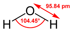
The figure below shows the general shape of the 3- to 6-site water models. The exact geometric parameters (the OH distance and the HOH angle) vary depending on the model.

2-site

A 2-site model of water based on the familiar three-site SPC model (see below) has been shown to predict the dielectric properties of water using site-renormalized molecular fluid theory. ^[7]

3-site

Three-site models have three interaction points corresponding to the three atoms of the water molecule. Each site has a point charge, and the site corresponding to the oxygen atom also has the Lennard-Jones parameters. Since 3-site models achieve a high computational efficiency, these are widely used for many applications of molecular dynamics simulations. Most of the models use a rigid geometry matching that of actual water molecules. An exception is the SPC model, which assumes an ideal tetrahedral shape (HOH angle of 109.47°) instead of the observed angle of 104.5°.

The table below lists the parameters for some 3-site models.

	TIPS [8]	SPC [9]	TIP3P [10]	SPC/E [11]
r(OH), Å	0.9572	1.0	0.9572	1.0
HOH, deg	104.52	109.47	104.52	109.47
A, 103 kcal Å12/mol	580.0	629.4	582.0	629.4
B, kcal Å6/mol	525.0	625.5	595.0	625.5
q(O)	−0.80	−0.82	−0.834	−0.8476
q(H)	+0.40	+0.41	+0.417	+0.4238

The SPC/E model adds an average polarization correction to the potential energy function:

${\displaystyle E_{\text{pol}}={\frac {1}{2}}\sum _{i}{\frac {(\mu -\mu ^{0})^{2}}{\alpha _{i}}},}$

where μ is the electric dipole moment of the effectively polarized water molecule (2.35 D for the SPC/E model), μ⁰ is the dipole moment of an isolated water molecule (1.85 D from experiment), and α_i is an isotropic polarizability constant, with a value of 1.608×10⁻⁴⁰  F·m². Since the charges in the model are constant, this correction just results in adding 1.25 kcal/mol (5.22 kJ/mol) to the total energy. The SPC/E model results in a better density and diffusion constant than the SPC model.

The TIP3P model implemented in the CHARMM force field is a slightly modified version of the original. The difference lies in the Lennard-Jones parameters: unlike TIP3P, the CHARMM version of the model places Lennard-Jones parameters on the hydrogen atoms too, in addition to the one on oxygen. The charges are not modified. ^[12] Three-site model (TIP3P) has better performance in calculating specific heats. ^[13]

Flexible SPC water model

Flexible SPC water model

The flexible simple point-charge water model (or flexible SPC water model) is a re-parametrization of the three-site SPC water model. ^{[14] [15]} The SPC model is rigid, whilst the flexible SPC model is flexible. In the model of Toukan and Rahman, the O–H stretching is made anharmonic, and thus the dynamical behavior is well described. This is one of the most accurate three-center water models without taking into account the polarization. In molecular dynamics simulations it gives the correct density and dielectric permittivity of water. ^[16]

Flexible SPC is implemented in the programs MDynaMix and Abalone.

Other models

• Ferguson (flexible SPC) ^[17]
• CVFF (flexible)
• MG (flexible and dissociative) ^[18]
• KKY potential (flexible model). ^[19]
• BLXL (smear charged potential). ^[20]

4-site

The four-site models have four interaction points by adding one dummy atom near of the oxygen along the bisector of the HOH angle of the three-site models (labeled M in the figure). The dummy atom only has a negative charge. This model improves the electrostatic distribution around the water molecule. The first model to use this approach was the Bernal–Fowler model published in 1933, ^[21] which may also be the earliest water model. However, the BF model doesn't reproduce well the bulk properties of water, such as density and heat of vaporization, and is thus of historical interest only. This is a consequence of the parameterization method; newer models, developed after modern computers became available, were parameterized by running Metropolis Monte Carlo or molecular dynamics simulations and adjusting the parameters until the bulk properties are reproduced well enough.

The TIP4P model, first published in 1983, is widely implemented in computational chemistry software packages and often used for the simulation of biomolecular systems. There have been subsequent reparameterizations of the TIP4P model for specific uses: the TIP4P-Ew model, for use with Ewald summation methods; the TIP4P/Ice, for simulation of solid water ice; TIP4P/2005, a general parameterization for simulating the entire phase diagram of condensed water; and TIP4PQ/2005, a similar model but designed to accurately describe the properties of solid and liquid water when quantum effects are included in the simulation. ^[22]

Most of the four-site water models use an OH distance and HOH angle which match those of the free water molecule. One exception is the OPC model, in which no geometry constraints are imposed other than the fundamental C_2v molecular symmetry of the water molecule. Instead, the point charges and their positions are optimized to best describe the electrostatics of the water molecule. OPC reproduces a comprehensive set of bulk properties more accurately than several of the commonly used rigid n-site water models. The OPC model is implemented within the AMBER force field.

	BF [21]	TIPS2 [23]	TIP4P [10]	TIP4P-Ew [24]	TIP4P/Ice [25]	TIP4P/2005 [26]	OPC [27]	TIP4P-D [28]
r(OH), Å	0.96	0.9572	0.9572	0.9572	0.9572	0.9572	0.8724	0.9572
HOH, deg	105.7	104.52	104.52	104.52	104.52	104.52	103.6	104.52
r(OM), Å	0.15	0.15	0.15	0.125	0.1577	0.1546	0.1594	0.1546
A, 103 kcal Å12/mol	560.4	695.0	600.0	656.1	857.9	731.3	865.1	904.7
B, kcal Å6/mol	837.0	600.0	610.0	653.5	850.5	736.0	858.1	900.0
q(M)	−0.98	−1.07	−1.04	−1.04844	−1.1794	−1.1128	−1.3582	−1.16
q(H)	+0.49	+0.535	+0.52	+0.52422	+0.5897	+0.5564	+0.6791	+0.58

Others:

• q-TIP4P/F (flexible) ^[29]
• TIP4P/2005f (flexible) ^[30]

5-site

The 5-site models place the negative charge on dummy atoms (labelled L) representing the lone pairs of the oxygen atom, with a tetrahedral-like geometry. An early model of these types was the BNS model of Ben-Naim and Stillinger, proposed in 1971,^{[ citation needed ]} soon succeeded by the ST2 model of Stillinger and Rahman in 1974. ^[31] Mainly due to their higher computational cost, five-site models were not developed much until 2000, when the TIP5P model of Mahoney and Jorgensen was published. ^[32] When compared with earlier models, the TIP5P model results in improvements in the geometry for the water dimer, a more "tetrahedral" water structure that better reproduces the experimental radial distribution functions from neutron diffraction, and the temperature of maximal density of water. The TIP5P-E model is a reparameterization of TIP5P for use with Ewald sums.

	BNS [31]	ST2 [31]	TIP5P [32]	TIP5P-E [33]
r(OH), Å	1.0	1.0	0.9572	0.9572
HOH, deg	109.47	109.47	104.52	104.52
r(OL), Å	1.0	0.8	0.70	0.70
LOL, deg	109.47	109.47	109.47	109.47
A, 103 kcal Å12/mol	77.4	238.7	544.5	554.3
B, kcal Å6/mol	153.8	268.9	590.3	628.2
q(L)	−0.19562	−0.2357	−0.241	−0.241
q(H)	+0.19562	+0.2357	+0.241	+0.241
RL, Å	2.0379	2.0160
RU, Å	3.1877	3.1287

Note, however, that the BNS and ST2 models do not use Coulomb's law directly for the electrostatic terms, but a modified version that is scaled down at short distances by multiplying it by the switching function S(r):

${\displaystyle S(r_{ij})={\begin{cases}0&{\text{if }}r_{ij}\leq R_{\text{L}},\\{\frac {(r_{ij}-R_{L})^{2}(3R_{\text{U}}-R_{\text{L}}-2r_{ij})}{(R_{\text{U}}-R_{\text{L}})^{2}}}&{\text{if }}R_{\text{L}}\leq r_{ij}\leq R_{\text{U}},\\1&{\text{if }}R_{\text{U}}\leq r_{ij}.\end{cases}}}$

Thus, the R_L and R_U parameters only apply to BNS and ST2.

6-site

Originally designed to study water/ice systems, a 6-site model that combines all the sites of the 4- and 5-site models was developed by Nada and van der Eerden. ^[34] Since it had a very high melting temperature ^[35] when employed under periodic electrostatic conditions (Ewald summation), a modified version was published later ^[36] optimized by using the Ewald method for estimating the Coulomb interaction.

Other

• The effect of explicit solute model on solute behavior in biomolecular simulations has been also extensively studied. It was shown that explicit water models affected the specific solvation and dynamics of unfolded peptides, while the conformational behavior and flexibility of folded peptides remained intact. ^[37]
• MB model. A more abstract model resembling the Mercedes-Benz logo that reproduces some features of water in two-dimensional systems. It is not used as such for simulations of "real" (i.e., three-dimensional) systems, but it is useful for qualitative studies and for educational purposes. ^[38]
• Coarse-grained models. One- and two-site models of water have also been developed. ^[39] In coarse-grain models, each site can represent several water molecules.
• Many-body models. Water models built using training-set configurations solved quantum mechanically, which then use machine learning protocols to extract potential-energy surfaces. These potential-energy surfaces are fed into MD simulations for an unprecedented degree of accuracy in computing physical properties of condensed phase systems. ^[40]
  • Another classification of many body models ^[41] is on the basis of the expansion of the underlying electrostatics, e.g., the SCME (Single Center Multipole Expansion) model ^[42]

Computational cost

The computational cost of a water simulation increases with the number of interaction sites in the water model. The CPU time is approximately proportional to the number of interatomic distances that need to be computed. For the 3-site model, 9 distances are required for each pair of water molecules (every atom of one molecule against every atom of the other molecule, or 3 × 3). For the 4-site model, 10 distances are required (every charged site with every charged site, plus the O–O interaction, or 3 × 3 + 1). For the 5-site model, 17 distances are required (4 × 4 + 1). Finally, for the 6-site model, 26 distances are required (5 × 5 + 1).

When using rigid water models in molecular dynamics, there is an additional cost associated with keeping the structure constrained, using constraint algorithms (although with bond lengths constrained it is often possible to increase the time step).

See also

• Water (properties)
• Water (data page)
• Water dimer
• Force field (chemistry)
• Comparison of force field implementations
• Molecular mechanics
• Molecular modelling
• Comparison of software for molecular mechanics modeling
• Solvent models

References

1. Skyner RE, McDonagh JL, Groom CR, van Mourik T, Mitchell JB (March 2015). "A review of methods for the calculation of solution free energies and the modelling of systems in solution" (PDF). Physical Chemistry Chemical Physics. 17 (9): 6174–91. Bibcode:2015PCCP...17.6174S. doi: 10.1039/C5CP00288E . PMID   25660403.
2. Allen MP, Tildesley DJ (1989). Computer Simulation of Liquids. Clarendon Press. ISBN   978-0-19-855645-9.
3. Kirby BJ. Micro- and Nanoscale Fluid Mechanics: Transport in Microfluidic Devices.
4. Swails JM, Roitberg AE (2013). "prmtop file of {A}mber" (PDF).
5. Swails JM (2013). Free energy simulations of complex biological systems at constant pH (PDF). University of Florida.
6. Case DA, Walker RC, Cheatham III TE, Simmerling CL, Roitberg A, Merz KM, et al. (April 2019). "Amber 2019 reference manual (covers Amber18 and AmberTools19)" (PDF).
7. Dyer KM, Perkyns JS, Stell G, Pettitt BM (2009). "Site-renormalised molecular fluid theory: on the utility of a two-site model of water". Molecular Physics. 107 (4–6): 423–431. Bibcode:2009MolPh.107..423D. doi:10.1080/00268970902845313. PMC   2777734 . PMID   19920881.
8. Jorgensen, William L. (1981). "Quantum and statistical mechanical studies of liquids. 10. Transferable intermolecular potential functions for water, alcohols, and ethers. Application to liquid water". Journal of the American Chemical Society. American Chemical Society (ACS). 103 (2): 335–340. doi:10.1021/ja00392a016. ISSN   0002-7863.
9. H. J. C. Berendsen, J. P. M. Postma, W. F. van Gunsteren, and J. Hermans, In Intermolecular Forces, edited by B. Pullman (Reidel, Dordrecht, 1981), p. 331.
10. Jorgensen WL, Chandrasekhar J, Madura JD, Impey RW, Klein ML (1983). "Comparison of simple potential functions for simulating liquid water". The Journal of Chemical Physics. 79 (2): 926–935. Bibcode:1983JChPh..79..926J. doi:10.1063/1.445869.
11. Berendsen HJ, Grigera JR, Straatsma TP (1987). "The missing term in effective pair potentials". The Journal of Physical Chemistry. 91 (24): 6269–6271. doi:10.1021/j100308a038.
12. MacKerell AD, Bashford D, Bellott M, Dunbrack RL, Evanseck JD, Field MJ, et al. (April 1998). "All-atom empirical potential for molecular modeling and dynamics studies of proteins". The Journal of Physical Chemistry B. 102 (18): 3586–616. doi:10.1021/jp973084f. PMID   24889800.
13. Mao Y, Zhang Y (2012). "Thermal conductivity, shear viscosity and specific heat of rigid water models". Chemical Physics Letters. 542: 37–41. Bibcode:2012CPL...542...37M. doi:10.1016/j.cplett.2012.05.044.
14. Toukan K, Rahman A (March 1985). "Molecular-dynamics study of atomic motions in water". Physical Review B. 31 (5): 2643–2648. Bibcode:1985PhRvB..31.2643T. doi:10.1103/PhysRevB.31.2643. PMID   9936106.
15. Berendsen HJ, Grigera JR, Straatsma TP (1987). "The missing term in effective pair potentials". Journal of Physical Chemistry . 91 (24): 6269–6271. doi:10.1021/j100308a038.
16. Praprotnik M, Janezic D, Mavri J (2004). "Temperature Dependence of Water Vibrational Spectrum: A Molecular Dynamics Simulation Study". Journal of Physical Chemistry A . 108 (50): 11056–11062. Bibcode:2004JPCA..10811056P. doi:10.1021/jp046158d.
17. Ferguson, David M. (April 1995). "Parameterization and evaluation of a flexible water model". Journal of Computational Chemistry. 16 (4): 501–511. doi:10.1002/jcc.540160413. S2CID   206038409 . Retrieved 28 July 2021.
18. MG model Archived 2016-03-04 at the Wayback Machine .
19. Kumagai N, Kawamura K, Yokokawa T (1994). "An Interatomic Potential Model for H2O: Applications to Water and Ice Polymorphs". Molecular Simulation. Informa UK Limited. 12 (3–6): 177–186. doi:10.1080/08927029408023028. ISSN   0892-7022.
20. Burnham CJ, Li J, Xantheas SS, Leslie M (1999). "The parametrization of a Thole-type all-atom polarizable water model from first principles and its application to the study of water clusters (n=2–21) and the phonon spectrum of ice Ih". The Journal of Chemical Physics. 110 (9): 4566–4581. Bibcode:1999JChPh.110.4566B. doi:10.1063/1.478797.
21. Bernal JD, Fowler RH (1933). "A Theory of Water and Ionic Solution, with Particular Reference to Hydrogen and Hydroxyl Ions". The Journal of Chemical Physics. 1 (8): 515. Bibcode:1933JChPh...1..515B. doi:10.1063/1.1749327.
22. McBride, C.; Vega, C.; Noya, E.G.; Ramirez, R.; Sese', L.M. (2009). "Quantum contributions in the ice phases: The path to a new empirical model for water—TIP4PQ/2005". J. Chem. Phys. 131 (2): 024506. arXiv: 0906.3967 . Bibcode:2009JChPh.131b4506M. doi:10.1063/1.3175694. PMID   19604003. S2CID   15505037.
23. Jorgensen (1982). "Revised TIPS for simulations of liquid water and aqueous solutions". The Journal of Chemical Physics. 77 (8): 4156–4163. Bibcode:1982JChPh..77.4156J. doi: 10.1063/1.444325 .
24. Horn HW, Swope WC, Pitera JW, Madura JD, Dick TJ, Hura GL, Head-Gordon T (May 2004). "Development of an improved four-site water model for biomolecular simulations: TIP4P-Ew". The Journal of Chemical Physics. 120 (20): 9665–78. Bibcode:2004JChPh.120.9665H. doi:10.1063/1.1683075. PMID   15267980. S2CID   39545298.
25. Abascal JL, Sanz E, García Fernández R, Vega C (June 2005). "A potential model for the study of ices and amorphous water: TIP4P/Ice". The Journal of Chemical Physics. 122 (23): 234511. Bibcode:2005JChPh.122w4511A. doi:10.1063/1.1931662. PMID   16008466. S2CID   8382245.
26. Abascal JL, Vega C (December 2005). "A general purpose model for the condensed phases of water: TIP4P/2005". The Journal of Chemical Physics. 123 (23): 234505. Bibcode:2005JChPh.123w4505A. doi:10.1063/1.2121687. PMID   16392929. S2CID   9757894.
27. Izadi S, Anandakrishnan R, Onufriev AV (November 2014). "Building Water Models: A Different Approach". The Journal of Physical Chemistry Letters. 5 (21): 3863–3871. arXiv: 1408.1679 . Bibcode:2014arXiv1408.1679I. doi:10.1021/jz501780a. PMC   4226301 . PMID   25400877.
28. Piana S, Donchev AG, Robustelli P, Shaw DE (April 2015). "Water dispersion interactions strongly influence simulated structural properties of disordered protein states". The Journal of Physical Chemistry B. 119 (16): 5113–23. doi: 10.1021/jp508971m . PMID   25764013.
29. Habershon, S.; Markland, T.E.; Manolopoulos, D.E. (2009). "Competing quantum effects in the dynamics of a flexible water model". J. Chem. Phys. 131 (2): 024501. arXiv: 1011.1047 . Bibcode:2009JChPh.131b4501H. doi:10.1063/1.3167790. PMID   19603998. S2CID   9095938.
30. Gonzalez, M.A.; Abascal, J.J.F. (2011). "A flexible model for water based on TIP4P/2005". J. Chem. Phys. 135 (22): 224516. Bibcode:2011JChPh.135v4516G. doi:10.1063/1.3663219. PMID   22168712.
31. Stillinger FH, Rahman A (1974). "Improved simulation of liquid water by molecular dynamics". The Journal of Chemical Physics. 60 (4): 1545–1557. Bibcode:1974JChPh..60.1545S. doi:10.1063/1.1681229. S2CID   96035805.
32. Mahoney MW, Jorgensen WL (2000). "A five-site model for liquid water and the reproduction of the density anomaly by rigid, nonpolarizable potential functions". The Journal of Chemical Physics. 112 (20): 8910–8922. Bibcode:2000JChPh.112.8910M. doi:10.1063/1.481505. S2CID   16367148.
33. Rick SW (April 2004). "A reoptimization of the five-site water potential (TIP5P) for use with Ewald sums". The Journal of Chemical Physics. 120 (13): 6085–93. Bibcode:2004JChPh.120.6085R. doi:10.1063/1.1652434. PMID   15267492.
34. Nada, H. (2003). "An intermolecular potential model for the simulation of ice and water near the melting point: A six-site model of H₂O". The Journal of Chemical Physics. 118 (16): 7401. Bibcode:2003JChPh.118.7401N. doi:10.1063/1.1562610.
35. Abascal JL, Fernández RG, Vega C, Carignano MA (October 2006). "The melting temperature of the six site potential model of water". The Journal of Chemical Physics. 125 (16): 166101. Bibcode:2006JChPh.125p6101A. doi:10.1063/1.2360276. PMID   17092145. S2CID   33883071.
36. Nada H (December 2016). "2O and a molecular dynamics simulation". The Journal of Chemical Physics. 145 (24): 244706. Bibcode:2016JChPh.145x4706N. doi:10.1063/1.4973000. PMID   28049310.
37. Florová P, Sklenovský P, Banáš P, Otyepka M (November 2010). "Explicit Water Models Affect the Specific Solvation and Dynamics of Unfolded Peptides While the Conformational Behavior and Flexibility of Folded Peptides Remain Intact". Journal of Chemical Theory and Computation. 6 (11): 3569–79. doi: 10.1021/ct1003687 . PMID   26617103.
38. Silverstein KA, Haymet AD, Dill KA (1998). "A Simple Model of Water and the Hydrophobic Effect". Journal of the American Chemical Society. 120 (13): 3166–3175. doi:10.1021/ja973029k.
39. Izvekov S, Voth GA (October 2005). "Multiscale coarse graining of liquid-state systems". The Journal of Chemical Physics. AIP Publishing. 123 (13): 134105. Bibcode:2005JChPh.123m4105I. doi:10.1063/1.2038787. PMID   16223273.
40. Medders GR, Paesani F (March 2015). "Infrared and Raman Spectroscopy of Liquid Water through "First-Principles" Many-Body Molecular Dynamics". Journal of Chemical Theory and Computation. 11 (3): 1145–54. doi:10.1021/ct501131j. PMID   26579763.
41. Cisneros GA, Wikfeldt KT, Ojamäe L, Lu J, Xu Y, Torabifard H, et al. (July 2016). "Modeling Molecular Interactions in Water: From Pairwise to Many-Body Potential Energy Functions". Chemical Reviews. 116 (13): 7501–28. doi:10.1021/acs.chemrev.5b00644. PMC   5450669 . PMID   27186804.
42. Wikfeldt KT, Batista ER, Vila FD, Jónsson H (October 2013). "A transferable H2O interaction potential based on a single center multipole expansion: SCME". Physical Chemistry Chemical Physics. 15 (39): 16542–56. arXiv: 1306.0327 . Bibcode:2013PCCP...1516542W. doi:10.1039/c3cp52097h. PMID   23949215. S2CID   15215071.