to generate a model of ten rays typically four rays more are added to the six rays model, these are ( and bouncing on both sides of the wall); This incorporate paths from one to three reflections: specifically, there is the LOS (Line of sight), GR (ground reflected), SW (single-wall reflected), DW (double-wall reflected), TW (triple-wall reflected), WG (wall-ground reflected) and GW (ground-wall reflected paths). Where each one of the paths bounces on both sides of the wall.
Experimentally, it has been demonstrated that the ten ray model simulates or can represent the propagation of signals through a dielectric canyon, in it which the rays that travel from a transmitter point to a receiver point bounce many times.
As example for this model it is assume: a rectilinear free space with two walls, one upper and the other lower, from which two vertical bases are positioned at their ends, these are the transmitting and receiving antennas that it's locate in such a way that their heights don't surpass the limits of the top wall; Achieved this the structure acts as free space for its functioning similar to that of a dielectric canyon of signals propagation, since the rays transmitted from the transmitting antenna will collide each side of the upper and lower walls infinity of times (for this example up to 3 reflections) until reaching the receiving antenna. During the course of the rays for each reflection they suffer, part of the energy of the signal is dissipated in each reflection, normally after the third reflection of said ray its resulting component which is a retro-reflected ray is insignificant with a negligible energy.[1]
Mathematical deduction
Analysis for antennas of heights different heights located in street's any point
For the mathematical modeling of the propagation of ten rays, One has in account a side view and this starts off modeling the two first rays (line by sight and his respective reflection), Considering that antennas have different heights, Then , and they have a direct distance d that separates the two antennas; The first ray is formed applying Pitágoras theorem:
The second ray or the reflected ray is made in a similar way to the first, but in this case the heights of the antennas to form the right angled triangle for the reflection of the height of the transmitter are added up.
In the deduction of the third ray it is necessary find the angle between the direct distance and the distance of line of view .
Viewing the model with a side view, it is necessary to find a flat distance between the transmitter and receiver called .
Now we deduce the remaining height of the wall from the height of the receiver called by the similarity of triangles:
By likeness of triangles we can deduce the distance from where collides the ray to wall until the perpendicular of the receiver called , getting:
The third ray is defined as a model of two-rays, by which is:
Taking a side view it is achieves to evidence the reflected ray that there in and is find as following manner:
As exist two rays that collide once on the wall, then is find the fifth ray, equating it to the third.
Similarly, is equalized the sixth ray with the fourth ray, since they have the same characteristics.
Side view of two transmitted beams reflected from one wall to the other side and reflected to the receiver on antennas of different heights at any point on the street.
To model the rays that collide with the wall twice, is used the Pythagoras theorem because of the direct distance and the sum of the distances between the receiver to each wall with double of distance of the transmitter to the wall , this divides on the angle formed between the direct distance and the reflected ray.
For the eighth ray is calculate a series of variables that allow to deduce the complete equation, which is composed by distances and heights that were found by likeness of triangles.
In first instance is take the flat distance between the wall of the second shock and the receiver:
Is found the flat distance between the transmitter and the wall in the first shock.
Finding the distance between the height of the wall of the second shock with respect to the first shock, is obtain:
Deducing also the distance between the height of the wall of the second shock with respect to the receiver:
Calculating the height of the wall where occurs the first hit:
Calculating the height of the wall where occurs the second shock:
With these parameters is calculate the equation for the eighth ray:
For the ninth ray, equation is the same as the seventh ray due to its characteristics:
For the tenth ray, the equation is the same as the eighth ray due to its reflected ray shape:
Losses for trajectory of free space
Modeling of the losses by free space trajectory in the 6-ray model when the distances of the wall and the heights are different.
Is considered a signal transmitted through free space to a receiver located at a distance d from the transmitter.
Assuming there are no obstacles between the transmitter and the receiver, the signal propagates along a straight line between the two. The beam model associated with this transmission is denominated line of sight (LOS), and the signal received corresponding is called the LOS signal or beam.[2]
The trajectory losses of the ten-ray model in free space is defined as:
Bessel functions, first defined by the mathematician Daniel Bernoulli and then generalized by Friedrich Bessel, are canonical solutions y(x) of Bessel's differential equation
In optics, a Gaussian beam is an idealized beam of electromagnetic radiation whose amplitude envelope in the transverse plane is given by a Gaussian function; this also implies a Gaussian intensity (irradiance) profile. This fundamental (or TEM00) transverse Gaussian mode describes the intended output of many lasers, as such a beam diverges less and can be focused better than any other. When a Gaussian beam is refocused by an ideal lens, a new Gaussian beam is produced. The electric and magnetic field amplitude profiles along a circular Gaussian beam of a given wavelength and polarization are determined by two parameters: the waistw0, which is a measure of the width of the beam at its narrowest point, and the position z relative to the waist.
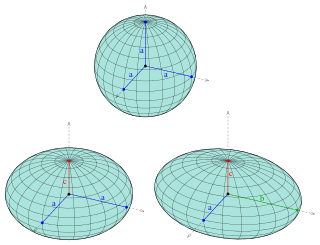
An ellipsoid is a surface that can be obtained from a sphere by deforming it by means of directional scalings, or more generally, of an affine transformation.
In mathematics, a Gaussian function, often simply referred to as a Gaussian, is a function of the base form
In mathematics, theta functions are special functions of several complex variables. They show up in many topics, including Abelian varieties, moduli spaces, quadratic forms, and solitons. As Grassmann algebras, they appear in quantum field theory.
In physics, a wave vector is a vector used in describing a wave, with a typical unit being cycle per metre. It has a magnitude and direction. Its magnitude is the wavenumber of the wave, and its direction is perpendicular to the wavefront. In isotropic media, this is also the direction of wave propagation.
The Friedmann equations, also known as the Friedmann–Lemaître (FL) equations, are a set of equations in physical cosmology that govern the expansion of space in homogeneous and isotropic models of the universe within the context of general relativity. They were first derived by Alexander Friedmann in 1922 from Einstein's field equations of gravitation for the Friedmann–Lemaître–Robertson–Walker metric and a perfect fluid with a given mass density ρ and pressure p. The equations for negative spatial curvature were given by Friedmann in 1924.
A Chapman function describes the integration of atmospheric absorption along a slant path on a spherical Earth, relative to the vertical case. It applies to any quantity with a concentration decreasing exponentially with increasing altitude. To a first approximation, valid at small zenith angles, the Chapman function for optical absorption is equal to
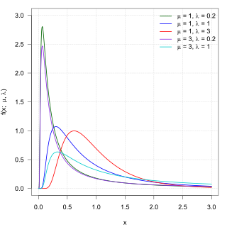
In probability theory, the inverse Gaussian distribution is a two-parameter family of continuous probability distributions with support on (0,∞).
In the mathematical discipline of graph theory, the expander walk sampling theorem intuitively states that sampling vertices in an expander graph by doing relatively short random walk can simulate sampling the vertices independently from a uniform distribution. The earliest version of this theorem is due to Ajtai, Komlós & Szemerédi (1987), and the more general version is typically attributed to Gillman (1998).
In mathematics, Gaussian measure is a Borel measure on finite-dimensional Euclidean space , closely related to the normal distribution in statistics. There is also a generalization to infinite-dimensional spaces. Gaussian measures are named after the German mathematician Carl Friedrich Gauss. One reason why Gaussian measures are so ubiquitous in probability theory is the central limit theorem. Loosely speaking, it states that if a random variable is obtained by summing a large number of independent random variables with variance 1, then has variance and its law is approximately Gaussian.
In mathematics, the Schur orthogonality relations, which were proven by Issai Schur through Schur's lemma, express a central fact about representations of finite groups. They admit a generalization to the case of compact groups in general, and in particular compact Lie groups, such as the rotation group SO(3).
A ratio distribution is a probability distribution constructed as the distribution of the ratio of random variables having two other known distributions. Given two random variables X and Y, the distribution of the random variable Z that is formed as the ratio Z = X/Y is a ratio distribution.
Contact mechanics is the study of the deformation of solids that touch each other at one or more points. A central distinction in contact mechanics is between stresses acting perpendicular to the contacting bodies' surfaces and frictional stresses acting tangentially between the surfaces. Normal contact mechanics or frictionless contact mechanics focuses on normal stresses caused by applied normal forces and by the adhesion present on surfaces in close contact, even if they are clean and dry. Frictional contact mechanics emphasizes the effect of friction forces.
Common integrals in quantum field theory are all variations and generalizations of Gaussian integrals to the complex plane and to multiple dimensions. Other integrals can be approximated by versions of the Gaussian integral. Fourier integrals are also considered.
In statistics, the Matérn covariance, also called the Matérn kernel, is a covariance function used in spatial statistics, geostatistics, machine learning, image analysis, and other applications of multivariate statistical analysis on metric spaces. It is named after the Swedish forestry statistician Bertil Matérn. It specifies the covariance between two measurements as a function of the distance between the points at which they are taken. Since the covariance only depends on distances between points, it is stationary. If the distance is Euclidean distance, the Matérn covariance is also isotropic.
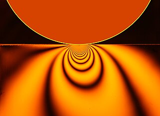
In optics, the Fraunhofer diffraction equation is used to model the diffraction of waves when the diffraction pattern is viewed at a long distance from the diffracting object, and also when it is viewed at the focal plane of an imaging lens.
The two-rays ground-reflection model is a multipath radio propagation model which predicts the path losses between a transmitting antenna and a receiving antenna when they are in line of sight (LOS). Generally, the two antenna each have different height. The received signal having two components, the LOS component and the reflection component formed predominantly by a single ground reflected wave.
The six-rays model is applied in an urban or indoor environment where a radio signal transmitted will encounter some objects that produce reflected, refracted or scattered copies of the transmitted signal. These are called multipath signal components, they are attenuated, delayed and shifted from the original signal (LOS) due to a finite number of reflectors with known location and dielectric properties, LOS and multipath signal are summed at the receiver.
In statistics, the complex Wishart distribution is a complex version of the Wishart distribution. It is the distribution of times the sample Hermitian covariance matrix of zero-mean independent Gaussian random variables. It has support for Hermitian positive definite matrices.
References
↑ Goldsmith, Andrea (2005). Wireless Communications. New York.: Cambridge University Press, ed. ISBN978-0521837163.
This page is based on this Wikipedia article Text is available under the CC BY-SA 4.0 license; additional terms may apply. Images, videos and audio are available under their respective licenses.