Six-rays model

Geometry of the six-ray model with location of antennas of equal heights at any point of the street in top view.

The six-rays model is applied in an urban or indoor environment where a radio signal transmitted will encounter some objects that produce reflected, refracted or scattered copies of the transmitted signal. These are called multipath signal components, they are attenuated, delayed and shifted from the original signal (LOS) due to a finite number of reflectors with known location and dielectric properties, LOS and multipath signal are summed at the receiver.

This model approach the propagation of electromagnetic waves by representing wavefront as simple particles. Thus reflection, refraction and scattering effects are approximated using simple geometric equation instead Maxwell's wave equations.[1]

The simplest model is two-rays which predicts signal variation resulting from a ground reflection interfering with the loss path. This model is applicable in isolated areas with some reflectors, such as rural roads or hallway.

The above two-rays approach can easily be extended to add as many rays as required. We may add rays bouncing off each side of a street in an urban corridor, leading to a six-rays model. The deduction of the six-rays model is presented below.

Mathematical deduction

Antennas of heights equal located in the center of the street

Angular view of the six rays transmitted with shock in the wall for antennas of equal height

Geometry of the 6-ray model with antenna location in the middle of the street

For the analysis of antennas with equal heights then ${\displaystyle h_{t}=h_{r}=h}$, determining that for the following two rays that are reflected once in the wall, the point in which they collide is equal to said height ${\displaystyle h}$. Also for each ray that is reflected in the wall, there is another ray that is reflected in the ground in a number equal to the reflections in the wall plus one, in these rays there are diagonal distances for each reflection and the sum of these distances is denominated ${\displaystyle d'}$.

Being located in the center of the street the distance between the antennas ${\displaystyle T_{X}}$ and ${\displaystyle R_{X}}$, the buildings and the width of the streets are equal in both sides so that ${\displaystyle w_{t1}=w_{r1}=w_{t2}=w_{r2}}$, defining thus a single distance ${\displaystyle w}$.

The mathematical model of propagation of six rays is based on the model of two rays, to find the equations of each ray involved. The distance ${\displaystyle d}$ that separates the two antennas, is equal to the first direct ray ${\displaystyle R_{0}}$ or line of sight (LOS), that is:

${\displaystyle R_{0}=d}$

For the ray reflected under ${\displaystyle R_{0}}$ applies the theorem of Pythagoras, in the right triangle that forms between the reflection of ${\displaystyle R_{0}}$ as the hypotenuse and the direct ray obtaining:

${\displaystyle R_{0}'={\sqrt {d^{2}+(2*h)^{2}}}}$

For ${\displaystyle R_{1}}$ the Pythagorean theorem is reapplied, knowing that one of the hinges is double the distances between the transmitter and the building due to the reflection of ${\displaystyle w}$ and the diagonal distance to the wall:

Side view of six rays transmitted with shock on the wall and wall mounted receiver for antennas of equal heigh

${\displaystyle R_{1}={\sqrt {d^{2}+(2*w)^{2}}}}$

For ${\displaystyle R_{1}}$ the second ray is multiplied twice but it is taken into account that the distance is half of the third ray to form the equivalent triangle considering that ${\displaystyle d_{1}}$ is the half of the distance of ${\displaystyle R_{1}}$ and these must be the half of the line of sight distance ${\displaystyle d}$:

${\displaystyle R_{1}'=2*{\sqrt {\left({\frac {R_{1}}{2}}\right)^{2}+(2h)^{2}}}}$

For ${\displaystyle R_{1}}$ y ${\displaystyle R_{2}}$ the deduction and the distances are equals, therefore:

${\displaystyle R_{2}=R_{1}}$

${\displaystyle R_{2}'=R_{1}'}$

Antennas of heights equal located in any point of the street

As the direct ray LOS does not vary and has not angular variation between the rays, the distance of the first two rays ${\displaystyle R_{0}}$ and ${\displaystyle R_{0}^{'}}$ of model does not vary and deduced according to the mathematic model for two rays. ^[1] For the other four rays it applies the next mathematical process:

${\displaystyle R_{1}}$ is obtained through a geometric analysis of the top view for the model and it applies the Pythagorean Theorem triangles, taking into account the distance between the wall and the antennas ${\displaystyle w_{t1}}$, ${\displaystyle w_{r1}}$, ${\displaystyle w_{t2}}$, ${\displaystyle w_{r2}}$ are different:

${\displaystyle R_{1}={\sqrt {d^{2}-(w_{t1}-w_{r2})^{2}+(w_{t1}+w_{t2}-w_{r2})^{2}}}}$

For likeness of triangles in the top view for model is determined the equation ${\displaystyle R_{1}}$:

${\displaystyle d'={\sqrt {d^{2}-(w_{t1}-w_{r2})^{2}}}}$

${\displaystyle x={\frac {(w_{r2}*R_{1})}{w_{r2}+w_{t2}+w_{t1}-w_{r2}}}}$

${\displaystyle R_{1}'={\sqrt {(R_{1}-x^{2})+(2*h^{2})}}+{\sqrt {(x)^{2}+(2*h)^{2}}}}$

For ${\displaystyle R_{1}}$ and ${\displaystyle R_{2}}$ the deduction and the distances are equal then:

${\displaystyle R_{2}=R_{1}}$

${\displaystyle R_{2}'=R_{1}'}$

Side view of antennas at different heights, unobstructed

Antennas of heights different located in the center of the street

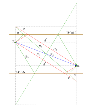
For antennas of different heights with rays that rebound in the wall, it is noted that the wall is the half point, where the two transmitted rays they fall on such wall. This wall has half the height between the height of the ${\displaystyle T_{X}}$ and ${\displaystyle R_{X}}$, it means smaller than the transmitter and higher than the receiver and this high is where the two rays impact in the point, then rebound to the receiver. The ray reflected leaves two reflections, one that it has the same high of the wall and the other the receiver, and the ray of the line of sight maintains the same direction between the ${\displaystyle T_{X}}$ and the ${\displaystyle R_{X}}$. The diagonal distance d´ that separates the two antennas divides in two distances through of the wall, one is called ${\displaystyle a}$ and the other ${\displaystyle d-a}$. ^[2]

Antennas of heights different located in any point of the street

For the mathematical model of six-ray propagation for antennas of different heights located at any point in the street, ${\displaystyle h_{t}\neq h_{r}}$, there is a direct distance ${\displaystyle d}$ that separates the two antennas, the first ray is formed by applying The Pythagorean theorem from the difference of heights of the antennas with respect to the line of sight:

${\displaystyle R_{0}={\sqrt {d^{2}+(h_{t}-h_{r})^{2}}}}$

Angular view of two rays transmitted with shock on the wall in antennas of different heights.

The second ray or reflected ray is calculated as the first ray but the heights of the antennas are added to form the right triangle.

${\displaystyle R_{0}'={\sqrt {d^{2}+(h_{t}+h_{r})^{2}}}}$

For deducing the third ray it is calculated the angle between the direct distance ${\displaystyle d}$ and the distance of line of sight ${\displaystyle R_{0}}$

${\displaystyle \cos \theta ={\frac {h_{t}-h_{r}}{R_{0}}}}$

Now deducing the height that subtraction of the wall with respect the height of the receiver called ${\displaystyle z}$ by similarity the triangles:

${\displaystyle {\frac {z}{a}}={\frac {h_{t}}{d'}}}$

${\displaystyle z={\frac {h_{t}*~a}{d'}}}$

By similarity of triangles it can deduce the distance where the ray hits the wall until the perpendicular of the receiver called a achieved:

${\displaystyle {\frac {a}{w^{t2}}}={\frac {d'}{w_{t1}+w_{r1}}}}$

${\displaystyle a={\frac {d'*w_{t2}}{\left(w_{t1}+w_{r1}\right)}}}$

${\displaystyle R_{1}={\frac {{\sqrt {(h_{t}-h_{r}-z)^{2}+(d'-a)^{2}}}+{\sqrt {z^{2}+a^{2}}}}{\cos \theta }}}$

By similarity of the triangles can be deduced the equation of the fourth ray:

${\displaystyle R_{1}'={\frac {{\sqrt {(h_{t}+h_{r}+z)^{2}+(d'-a)^{2}}}+{\sqrt {(2h_{r}+z)^{2}+a^{2}}}}{\cos \theta }}}$

For ${\displaystyle R_{1}}$ y ${\displaystyle R_{2}}$ the deduction and the distances are equal, therefore:

${\displaystyle R_{2}=R_{1}}$

${\displaystyle R_{2}'=R_{1}'}$

Free-space path loss on the model

Free-space path loss on the model of six-rays.

Consider a transmitted signal in the free space a receptor located a distance d of the transmitter. One may add rays bouncing off each side of a street in an urban corridor, leading to a six-rays model, with rays ${\displaystyle R_{0}}$, ${\displaystyle R_{1}}$ and ${\displaystyle R_{2}}$ each one having a direct and a ground bouncing ray. ^[3]

An important assumption must be made to simplify the model: ${\displaystyle T}$ is small compared to the symbol length of the useful information, that is ${\displaystyle s(t)=s(t-T)}$. For the rays rebound outside the earth and on each side of the street, this assumption is fairly safe, but in general will have remembered that these assumptions mean the dispersion of delays (diffusion of the values ${\displaystyle T}$) is smaller than symbols speed of transmission.

Free-space path loss of six rays model is defined as:

${\displaystyle p_{0}(t)={\sqrt {(G_{i}G_{r})}}{\frac {\lambda }{4\pi }}\left({\frac {\exp(j*2\pi *R_{0}/{\lambda })}{R_{0}}}+\Gamma {\frac {\exp(j*2\pi *R_{0}'/{\lambda })}{R_{0}'}}\right)}$

${\displaystyle p_{1}(t)={\sqrt {(G_{i}G_{r})}}{\frac {\lambda }{4\pi }}~\Gamma _{1}\left({\frac {\exp(j*2\pi *R_{1}/{\lambda })}{R_{1}}}+\Gamma {\frac {\exp(j*2\pi *R_{1}'/{\lambda })}{R_{1}'}}\right)}$

${\displaystyle p_{2}(t)={\sqrt {(G_{i}G_{r})}}{\frac {\lambda }{4\pi }}~\Gamma _{1}\left({\frac {\exp(j*2\pi *R_{2}/{\lambda })}{R_{2}}}+\Gamma {\frac {\exp(j*2\pi *R_{2}'/{\lambda })}{R_{2}'}}\right)}$

${\displaystyle P_{l}~(dB)=20\log \left|~\sum _{i=0}^{N}P_{i}~\right|}$

${\displaystyle {\lambda }=}$${\displaystyle {c \over f}}$ is the wavelength.

${\displaystyle T=}$ Is the time difference between the two paths.

${\displaystyle \Gamma =}$ Is the coefficient of ground reflection.

${\displaystyle G_{i}=}$ Gain of the transmitter.

${\displaystyle G_{r}=}$ Receiver gain.

See also

• Two-ray ground-reflection model
• Ten-rays model
• Ray tracing (physics)

References

1. T.Rappaport (2002). Wireless Communications: Principles and Practice . Upper Saddle River, N.J.: Prentice Hall. ISBN   978-0137192878.
2. A. J. Rustako, Jr., Noach Amitay, G. J. Owens, R.S. Roman. (1991). Radio Propagation at Microwave Frequencies for Line-of-Sight Microcellular Mobile and Personal Communications.
3. Schwengler, Thomas (2016). Wireless & Cellular Communications Class Notes for TLEN-5510-Fall. Universidad de Colorado. pp.  http://morse.colorado.edu/~tlen5510/text/classwebch3.html. Chapter 3: Radio Propagation Modeling

References

↑ Goldsmith, Andrea (2005). Wireless communications. Cambridge: Cambridge University Press. ISBN978-0-521-83716-3.