Partially linear model

Last updated

A partially linear model is a form of semiparametric model, since it contains parametric and nonparametric elements. Application of the least squares estimators is available to partially linear model, if the hypothesis of the known of nonparametric element is valid. Partially linear equations were first used in the analysis of the relationship between temperature and usage of electricity by Engle, Granger, Rice and Weiss (1986) [1] . Typical application of partially linear model in the field of Microeconomics is presented by Tripathi in the case of profitability of firm's production in 1997. Also, partially linear model applied successfully in some other academic field. In 1994, Zeger and Diggle introduced partially linear model into biometrics. In environmental science, Parda-Sanchez et al. used partially linear model to analysis collected data in 2000. So far, partially linear model was optimized in many other statistic methods. In 1988, Robinson applied Nadaraya-Waston kernel estimator to test the nonparametric element to build a least-squares estimator  After that, in 1997, local linear method was found by Truong.

Contents

Partially linear model

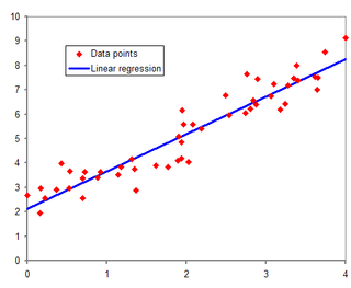
Regression,2009-12-01.jpg

Synopsis

Algebra equation

The algebra expression of partially linear model is written as:

[2]

Equation components outline

and : Vectors of explanatory variables. Independently random or fixed distributed variables.

: To be measured Parameter.

: The random error in statistics with 0 mean.

: To be measured part in partially linear model.

Assumption [2]

Wolfgang, Hua Liang and Jiti Gao consider the assumptions and remarks of partially linear model under fixed and random design conditions.

When randomly distributed, introduce

and (1)

is smaller than positive infinity when t value between 0 and 1, and the sum of covariance of  is positive. The random errors µ are independent of ,

When and Ti are fixed distributed, valued between 0 and 1, and satisfies , where factor i values between 1 and n, and factor j value between 1 and p, Error factor satisfies, .

The least square (LS) estimators [2]

The precondition of application of the least squares estimators is the existence of nonparametric component, and running at random distributed and fixed distributed cases.

Engle, Granger, Rice and Weiss's (1986) smoothing model should be first introduced, before applying the least squares estimators. The algebra function of their model is expressed as (2).

Wolfgang, Liang and Gao (1988) make an assumption that the pair (ß,g) satisfies (3).

This means that for all 1≤i≤n, .

So, .

Under random distributed case, Wolfgang, Hua Liang and Jiti Gao assume that for all 1 ≤ i ≤ n, (4)

so, , due to is a positive number, as function (1) proved. So, established for all 1≤i≤n and j equals to 1 and 2 when .

Under fixed distributed case, By parameterizing factor  from smoothing model (2) as where .

By making same assumption as (4), which follows from assumption (1), and under the fact of .

Assuming factors (i here are positive integers) satisfies and establish positive weight functions . Any estimators of , for every , we have . By applying LS criterion, the LS estimator of . The nonparametric estimator of   is expressed as . So, When the random errors are identically distributed, the estimators of variance  is expressed as, .

History and applications of partially linear model

The real-world application of partially linear model was first considered for analyzing data by Engle, Granger, Rice and Weiss in 1986. [2]

In their point of view, the relevance between temperature and the consumption of electricity cannot be expressed in a linear model, because there are massive of confounding factors, such as average income, goods price, consumer purchase ability and some other economic activities. Some of the factors are relevance with each other and might influence the observed result. Therefore, they introduced partially linear model, which contained both with parametric and nonparametric factors. The partially linear model enables and simplifies the linear transformation of data (Engle, Granger, Rice and Weiss, 1986). They also applied the smoothing spline technique for their research.

There was a case of application of partially linear model in biometrics by Zeger and Diggle in 1994. The research objective of their paper is the evolution period cycle of CD4 cell amounts in HIV (Human immune-deficiency virus) seroconverters (Zeger and Diggle, 1994). [3] CD4 cell plays a significant role in immune function in human body. Zeger and Diggle aimed to assess the proceed of disease by measuring the changing amount of CD4 cells. The number of CD4 cell is associated with body age and smoking behavior and so on. To clear the group of observation data in their experiment, Zeger and Diggle applied partially linear model for their work. Partially linear model primarily contributes to the estimation of average loss time of CD4 cells and adjusts the time dependence of some other covariables in order to simplify the proceed of data comparison, and also, the partially linear model characterizes the deviation of typical curve for their observed group to estimate the progression curve of the changing amount of CD4 cell. The deviation, granted by partially linear model, potentially helps to recognize the observed targets who had a slow progression on the amounting change of CD4 cells. 

In 1999, Schmalensee and Stoker (1999) have used partially linear model in the field of economics. The independent variable of their research is the demand for gasoline in The United States. The primary research target in their paper is the relationship between gasoline consumption and long-run income elasticity in the U.S. Similarly, there are also massive of confounding variables, which might mutually affect. Hence, Schmalemsee and Stoker chose to deal with the issues of linear transformation of data between parametric and nonparametric by applying partially linear model. [4]

In the field of environment science, Prada-Sanchez used partially linear model to predict the sulfur dioxide pollution in 2000 (Prada-Sanchez, 2000), [5] and in the next year, Lin and Carroll applied partially linear model for clustered data (Lin and Carroall, 2001). [6]

Development of partially linear model

According to Liang's paper in 2010 (Liang, 2010), The smoothing spline technique was introduced in partially linear model by Engle, Heckman and Rice in 1986. After that, Robinson found an available LS estimator for nonparametric factors in partially linear model in 1988. At the same year, profile LS method was recommended by Speckman. [7]

Other econometrics tools in partially linear model

Kernel regression also was introduced in partially linear model. The local constant method, which is developed by Speckman, and local linear techniques, which was found by Hamilton and Truong in 1997 and was revised by Opsomer and Ruppert in 1997, are all included in kernel regression. Green et al., Opsomer and Ruppert found that one of the significant characteristic of kernel-based methods is that under-smoothing has been taken in order to find root-n estimator of beta. However, Speckman's research in 1988 and Severini's and Staniswalis's research in 1994 proved that those restriction might be canceled.

Bandwidth selection in partially linear model [7]

Bandwidth selection in partially linear model is a confusing issue. Liang addressed a possible solution for this bandwidth selection in his literature by applying profile-kernel based method and backfitting methods. Also the necessity of undersmoothing for backfitting method and the reason why profile-kernel based method can work out the optimal bandwidth selection were justified by Liang. The general computation strategy is applied in Liang's literature for estimating nonparametric function. Moreover, the penalized spline method for partially linear models and intensive simulation experiments were introduced to discover the numerical feature of the penalized spline method, profile and backfitting methods.

Kernel-based profile and backfitting method [7]

By introducing

Following with

The intuitive estimator of ß can be defined as the LS estimator after appropriately estimating and .

Then, for all random vector variable , assume is a kernel regression estimator of . Let . For example, . Denote X,g and T similarly. Let . So

The profile-kernel based estimators solves,

where are kernel estimators of mx and my.

The penalized spline method [7]

The penalized spline method was developed by Eilers and Marx in 1996. Ruppert and Carroll in 2000 and Brumback, Ruppert and Wand in 1999 employed this method in LME framework.

Assuming function can be estimated by

where is an integer, and are fixed knots, Denote Consider . The penalized spline estimator is defined as follow

Where is a smoothing parameter.

As Brumback et al. mentioned in 1999, [8] the estimator is same as the estimator of based on LME model.

,

where ,

Where , and . The matrix shows the penalized spline smoother for up above framework.

Related Research Articles

<span class="mw-page-title-main">Least squares</span> Approximation method in statistics

The method of least squares is a parameter estimation method in regression analysis based on minimizing the sum of the squares of the residuals made in the results of each individual equation.

In statistics, the Gauss–Markov theorem states that the ordinary least squares (OLS) estimator has the lowest sampling variance within the class of linear unbiased estimators, if the errors in the linear regression model are uncorrelated, have equal variances and expectation value of zero. The errors do not need to be normal for the theorem to apply, nor do they need to be independent and identically distributed.

<span class="mw-page-title-main">Spearman's rank correlation coefficient</span> Nonparametric measure of rank correlation

In statistics, Spearman's rank correlation coefficient or Spearman's ρ, named after Charles Spearman and often denoted by the Greek letter (rho) or as , is a nonparametric measure of rank correlation. It assesses how well the relationship between two variables can be described using a monotonic function.

Simultaneous equations models are a type of statistical model in which the dependent variables are functions of other dependent variables, rather than just independent variables. This means some of the explanatory variables are jointly determined with the dependent variable, which in economics usually is the consequence of some underlying equilibrium mechanism. Take the typical supply and demand model: whilst typically one would determine the quantity supplied and demanded to be a function of the price set by the market, it is also possible for the reverse to be true, where producers observe the quantity that consumers demand and then set the price.
<span class="mw-page-title-main">Regression analysis</span> Set of statistical processes for estimating the relationships among variables

In statistical modeling, regression analysis is a set of statistical processes for estimating the relationships between a dependent variable and one or more independent variables. The most common form of regression analysis is linear regression, in which one finds the line that most closely fits the data according to a specific mathematical criterion. For example, the method of ordinary least squares computes the unique line that minimizes the sum of squared differences between the true data and that line. For specific mathematical reasons, this allows the researcher to estimate the conditional expectation of the dependent variable when the independent variables take on a given set of values. Less common forms of regression use slightly different procedures to estimate alternative location parameters or estimate the conditional expectation across a broader collection of non-linear models.

In statistics, omitted-variable bias (OVB) occurs when a statistical model leaves out one or more relevant variables. The bias results in the model attributing the effect of the missing variables to those that were included.

In statistics, the theory of minimum norm quadratic unbiased estimation (MINQUE) was developed by C. R. Rao. MINQUE is a theory alongside other estimation methods in estimation theory, such as the method of moments or maximum likelihood estimation. Similar to the theory of best linear unbiased estimation, MINQUE is specifically concerned with linear regression models. The method was originally conceived to estimate heteroscedastic error variance in multiple linear regression. MINQUE estimators also provide an alternative to maximum likelihood estimators or restricted maximum likelihood estimators for variance components in mixed effects models. MINQUE estimators are quadratic forms of the response variable and are used to estimate a linear function of the variances.

In statistics, a probit model is a type of regression where the dependent variable can take only two values, for example married or not married. The word is a portmanteau, coming from probability + unit. The purpose of the model is to estimate the probability that an observation with particular characteristics will fall into a specific one of the categories; moreover, classifying observations based on their predicted probabilities is a type of binary classification model.

In statistics, ordinary least squares (OLS) is a type of linear least squares method for choosing the unknown parameters in a linear regression model by the principle of least squares: minimizing the sum of the squares of the differences between the observed dependent variable in the input dataset and the output of the (linear) function of the independent variable.

<span class="mw-page-title-main">Simple linear regression</span> Linear regression model with a single explanatory variable

In statistics, simple linear regression (SLR) is a linear regression model with a single explanatory variable. That is, it concerns two-dimensional sample points with one independent variable and one dependent variable and finds a linear function that, as accurately as possible, predicts the dependent variable values as a function of the independent variable. The adjective simple refers to the fact that the outcome variable is related to a single predictor.

In mathematics, in particular in algebraic geometry and differential geometry, Dolbeault cohomology (named after Pierre Dolbeault) is an analog of de Rham cohomology for complex manifolds. Let M be a complex manifold. Then the Dolbeault cohomology groups depend on a pair of integers p and q and are realized as a subquotient of the space of complex differential forms of degree (p,q).

In statistics, semiparametric regression includes regression models that combine parametric and nonparametric models. They are often used in situations where the fully nonparametric model may not perform well or when the researcher wants to use a parametric model but the functional form with respect to a subset of the regressors or the density of the errors is not known. Semiparametric regression models are a particular type of semiparametric modelling and, since semiparametric models contain a parametric component, they rely on parametric assumptions and may be misspecified and inconsistent, just like a fully parametric model.

In statistics, the Kendall rank correlation coefficient, commonly referred to as Kendall's τ coefficient, is a statistic used to measure the ordinal association between two measured quantities. A τ test is a non-parametric hypothesis test for statistical dependence based on the τ coefficient. It is a measure of rank correlation: the similarity of the orderings of the data when ranked by each of the quantities. It is named after Maurice Kendall, who developed it in 1938, though Gustav Fechner had proposed a similar measure in the context of time series in 1897.

<span class="mw-page-title-main">Quantile regression</span> Statistics concept

Quantile regression is a type of regression analysis used in statistics and econometrics. Whereas the method of least squares estimates the conditional mean of the response variable across values of the predictor variables, quantile regression estimates the conditional median of the response variable. Quantile regression is an extension of linear regression used when the conditions of linear regression are not met.

In statistics, principal component regression (PCR) is a regression analysis technique that is based on principal component analysis (PCA). More specifically, PCR is used for estimating the unknown regression coefficients in a standard linear regression model.

Smoothing splines are function estimates, , obtained from a set of noisy observations of the target , in order to balance a measure of goodness of fit of to with a derivative based measure of the smoothness of . They provide a means for smoothing noisy data. The most familiar example is the cubic smoothing spline, but there are many other possibilities, including for the case where is a vector quantity.

In statistics and machine learning, lasso is a regression analysis method that performs both variable selection and regularization in order to enhance the prediction accuracy and interpretability of the resulting statistical model. The lasso method assumes that the coefficients of the linear model are sparse, meaning that few of them are non-zero. It was originally introduced in geophysics, and later by Robert Tibshirani, who coined the term.

In statistics and econometrics, the maximum score estimator is a nonparametric estimator for discrete choice models developed by Charles Manski in 1975. Unlike the multinomial probit and multinomial logit estimators, it makes no assumptions about the distribution of the unobservable part of utility. However, its statistical properties are more complicated than the multinomial probit and logit models, making statistical inference difficult. To address these issues, Joel Horowitz proposed a variant, called the smoothed maximum score estimator.

In statistics, linear regression is a statistical model which estimates the linear relationship between a scalar response and one or more explanatory variables. The case of one explanatory variable is called simple linear regression; for more than one, the process is called multiple linear regression. This term is distinct from multivariate linear regression, where multiple correlated dependent variables are predicted, rather than a single scalar variable. If the explanatory variables are measured with error then errors-in-variables models are required, also known as measurement error models.

Hypertabastic survival models were introduced in 2007 by Mohammad Tabatabai, Zoran Bursac, David Williams, and Karan Singh. This distribution can be used to analyze time-to-event data in biomedical and public health areas and normally called survival analysis. In engineering, the time-to-event analysis is referred to as reliability theory and in business and economics it is called duration analysis. Other fields may use different names for the same analysis. These survival models are applicable in many fields such as biomedical, behavioral science, social science, statistics, medicine, bioinformatics, medical informatics, data science especially in machine learning, computational biology, business economics, engineering, and commercial entities. They not only look at the time to event, but whether or not the event occurred. These time-to-event models can be applied in a variety of applications for instance, time after diagnosis of cancer until death, comparison of individualized treatment with standard care in cancer research, time until an individual defaults on loans, relapsed time for drug and smoking cessation, time until property sold after being put on the market, time until an individual upgrades to a new phone, time until job relocation, time until bones receive microscopic fractures when undergoing different stress levels, time from marriage until divorce, time until infection due to catheter, and time from bridge completion until first repair.

References

  1. Engle, Robert F.; Granger, C. W. J.; Rice, John; Weiss, Andrew (1986). "Semiparametric Estimates of the Relation Between Weather and Electricity Sales". Journal of the American Statistical Association. 81 (394): 310–20. doi:10.2307/2289218.
  2. 1 2 3 4 Hardle, Liang, JiTi, WolfGang, Hua, Gao (2000). Partially linear model. PHYSICA-VERLAG.{{cite book}}: CS1 maint: multiple names: authors list (link)
  3. Zeger, Scott L.; Diggle, Peter J. (1994). "Semiparametric Models for Longitudinal Data with Application to CD4 Cell Numbers in HIV Seroconverters". Biometrics. 50 (3): 689–699. doi:10.2307/2532783. ISSN   0006-341X. JSTOR   2532783. PMID   7981395.
  4. Schmalensee, Richard; Stoker, Thomas M. (1999). "Household Gasoline Demand in the United States" (PDF). Econometrica. 67 (3): 645–662. doi:10.1111/1468-0262.00041. hdl: 1721.1/50215 . ISSN   1468-0262.
  5. Prada‐Sánchez, J. M.; Febrero‐Bande, M.; Cotos‐Yáñez, T.; González‐Manteiga, W.; Bermúdez‐Cela, J. L.; Lucas‐Domínguez, T. (2000). "Prediction of SO2 pollution incidents near a power station using partially linear models and an historical matrix of predictor-response vectors". Environmetrics. 11 (2): 209–225. doi:10.1002/(SICI)1099-095X(200003/04)11:2<209::AID-ENV403>3.0.CO;2-Z. ISSN   1099-095X.
  6. Carroll, Raymond J.; Lin, Xihong (2001-12-01). "Semiparametric regression for clustered data". Biometrika. 88 (4): 1179–1185. doi:10.1093/biomet/88.4.1179. ISSN   0006-3444.
  7. 1 2 3 4 Liang, Hua (2006-02-10). "Estimation in Partially Linear Models and Numerical Comparisons". Computational Statistics & Data Analysis. 50 (3): 675–687. doi:10.1016/j.csda.2004.10.007. ISSN   0167-9473. PMC   2824448 . PMID   20174596.
  8. Brumback, Babette A.; Ruppert, David; Wand, M. P. (1999). "Variable Selection and Function Estimation in Additive Nonparametric Regression Using a Data-Based Prior: Comment". Journal of the American Statistical Association. 94 (447): 794–797. doi:10.2307/2669991. ISSN   0162-1459. JSTOR   2669991.