Multivariate statistics is a subdivision of statistics encompassing the simultaneous observation and analysis of more than one outcome variable. Multivariate statistics concerns understanding the different aims and background of each of the different forms of multivariate analysis, and how they relate to each other. The practical application of multivariate statistics to a particular problem may involve several types of univariate and multivariate analyses in order to understand the relationships between variables and their relevance to the problem being studied.

In statistics, correlation or dependence is any statistical relationship, whether causal or not, between two random variables or bivariate data. Although in the broadest sense, "correlation" may indicate any type of association, in statistics it normally refers to the degree to which a pair of variables are linearly related. Familiar examples of dependent phenomena include the correlation between the height of parents and their offspring, and the correlation between the price of a good and the quantity the consumers are willing to purchase, as it is depicted in the so-called demand curve.
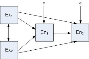
Simultaneous equations models are a type of statistical model in which the dependent variables are functions of other dependent variables, rather than just independent variables. This means some of the explanatory variables are jointly determined with the dependent variable, which in economics usually is the consequence of some underlying equilibrium mechanism. Take the typical supply and demand model: whilst typically one would determine the quantity supplied and demanded to be a function of the price set by the market, it is also possible for the reverse to be true, where producers observe the quantity that consumers demand and then set the price.

In statistics, the coefficient of determination, denoted R2 or r2 and pronounced "R squared", is the proportion of the variation in the dependent variable that is predictable from the independent variable(s).
In statistics, econometrics, epidemiology and related disciplines, the method of instrumental variables (IV) is used to estimate causal relationships when controlled experiments are not feasible or when a treatment is not successfully delivered to every unit in a randomized experiment. Intuitively, IVs are used when an explanatory variable of interest is correlated with the error term, in which case ordinary least squares and ANOVA give biased results. A valid instrument induces changes in the explanatory variable but has no independent effect on the dependent variable, allowing a researcher to uncover the causal effect of the explanatory variable on the dependent variable.
In econometrics, endogeneity broadly refers to situations in which an explanatory variable is correlated with the error term. The distinction between endogenous and exogenous variables originated in simultaneous equations models, where one separates variables whose values are determined by the model from variables which are predetermined; ignoring simultaneity in the estimation leads to biased estimates as it violates the exogeneity assumption of the Gauss–Markov theorem. The problem of endogeneity is often ignored by researchers conducting non-experimental research and doing so precludes making policy recommendations. Instrumental variable techniques are commonly used to address this problem.
Structural equation modeling (SEM) is a label for a diverse set of methods used by scientists in both experimental and observational research across the sciences, business, and other fields. It is used most in the social and behavioral sciences. A definition of SEM is difficult without reference to highly technical language, but a good starting place is the name itself.
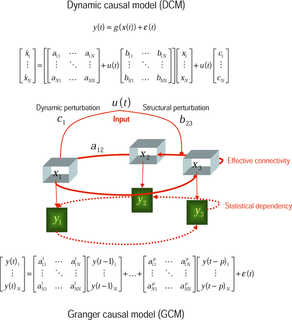
Vector autoregression (VAR) is a statistical model used to capture the relationship between multiple quantities as they change over time. VAR is a type of stochastic process model. VAR models generalize the single-variable (univariate) autoregressive model by allowing for multivariate time series. VAR models are often used in economics and the natural sciences.
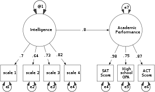
Path coefficients are standardized versions of linear regression weights which can be used in examining the possible causal linkage between statistical variables in the structural equation modeling approach. The standardization involves multiplying the ordinary regression coefficient by the standard deviations of the corresponding explanatory variable: these can then be compared to assess the relative effects of the variables within the fitted regression model. The idea of standardization can be extended to apply to partial regression coefficients.
In psychology, discriminant validity tests whether concepts or measurements that are not supposed to be related are actually unrelated.
In the philosophy of science, a causal model is a conceptual model that describes the causal mechanisms of a system. Causal models can improve study designs by providing clear rules for deciding which independent variables need to be included/controlled for.

In statistics, a mediation model seeks to identify and explain the mechanism or process that underlies an observed relationship between an independent variable and a dependent variable via the inclusion of a third hypothetical variable, known as a mediator variable. Rather than a direct causal relationship between the independent variable and the dependent variable, a mediation model proposes that the independent variable influences the mediator variable, which in turn influences the dependent variable. Thus, the mediator variable serves to clarify the nature of the relationship between the independent and dependent variables.
In statistics, confirmatory factor analysis (CFA) is a special form of factor analysis, most commonly used in social research. It is used to test whether measures of a construct are consistent with a researcher's understanding of the nature of that construct. As such, the objective of confirmatory factor analysis is to test whether the data fit a hypothesized measurement model. This hypothesized model is based on theory and/or previous analytic research. CFA was first developed by Jöreskog (1969) and has built upon and replaced older methods of analyzing construct validity such as the MTMM Matrix as described in Campbell & Fiske (1959).
One application of multilevel modeling (MLM) is the analysis of repeated measures data. Multilevel modeling for repeated measures data is most often discussed in the context of modeling change over time ; however, it may also be used for repeated measures data in which time is not a factor.
In statistics, econometrics, epidemiology, genetics and related disciplines, causal graphs are probabilistic graphical models used to encode assumptions about the data-generating process.
Control functions are statistical methods to correct for endogeneity problems by modelling the endogeneity in the error term. The approach thereby differs in important ways from other models that try to account for the same econometric problem. Instrumental variables, for example, attempt to model the endogenous variable X as an often invertible model with respect to a relevant and exogenous instrument Z. Panel analysis uses special data properties to difference out unobserved heterogeneity that is assumed to be fixed over time.

WarpPLS is a software with graphical user interface for variance-based and factor-based structural equation modeling (SEM) using the partial least squares and factor-based methods. The software can be used in empirical research to analyse collected data and test hypothesized relationships. Since it runs on the MATLAB Compiler Runtime, it does not require the MATLAB software development application to be installed; and can be installed and used on various operating systems in addition to Windows, with virtual installations.

In statistics, average variance extracted (AVE) is a measure of the amount of variance that is captured by a construct in relation to the amount of variance due to measurement error.
In statistics, confirmatory composite analysis (CCA) is a sub-type of structural equation modeling (SEM). Although, historically, CCA emerged from a re-orientation and re-start of partial least squares path modeling (PLS-PM), it has become an independent approach and the two should not be confused. In many ways it is similar to, but also quite distinct from confirmatory factor analysis (CFA). It shares with CFA the process of model specification, model identification, model estimation, and model assessment. However, in contrast to CFA which always assumes the existence of latent variables, in CCA all variables can be observable, with their interrelationships expressed in terms of composites, i.e., linear compounds of subsets of the variables. The composites are treated as the fundamental objects and path diagrams can be used to illustrate their relationships. This makes CCA particularly useful for disciplines examining theoretical concepts that are designed to attain certain goals, so-called artifacts, and their interplay with theoretical concepts of behavioral sciences.