Analysis of variance (ANOVA) is a collection of statistical models and their associated estimation procedures used to analyze the differences among means. ANOVA was developed by the statistician Ronald Fisher. ANOVA is based on the law of total variance, where the observed variance in a particular variable is partitioned into components attributable to different sources of variation. In its simplest form, ANOVA provides a statistical test of whether two or more population means are equal, and therefore generalizes the t-test beyond two means. In other words, the ANOVA is used to test the difference between two or more means.

In statistics, correlation or dependence is any statistical relationship, whether causal or not, between two random variables or bivariate data. Although in the broadest sense, "correlation" may indicate any type of association, in statistics it usually refers to the degree to which a pair of variables are linearly related. Familiar examples of dependent phenomena include the correlation between the height of parents and their offspring, and the correlation between the price of a good and the quantity the consumers are willing to purchase, as it is depicted in the so-called demand curve.

In statistics, the Pearson correlation coefficient (PCC) is a correlation coefficient that measures linear correlation between two sets of data. It is the ratio between the covariance of two variables and the product of their standard deviations; thus, it is essentially a normalized measurement of the covariance, such that the result always has a value between −1 and 1. As with covariance itself, the measure can only reflect a linear correlation of variables, and ignores many other types of relationships or correlations. As a simple example, one would expect the age and height of a sample of teenagers from a high school to have a Pearson correlation coefficient significantly greater than 0, but less than 1.

In statistics, Spearman's rank correlation coefficient or Spearman's ρ, named after Charles Spearman and often denoted by the Greek letter (rho) or as , is a nonparametric measure of rank correlation. It assesses how well the relationship between two variables can be described using a monotonic function.
In statistics, the power of a binary hypothesis test is the probability that the test correctly rejects the null hypothesis when a specific alternative hypothesis is true. It is commonly denoted by , and represents the chances of a true positive detection conditional on the actual existence of an effect to detect. Statistical power ranges from 0 to 1, and as the power of a test increases, the probability of making a type II error by wrongly failing to reject the null hypothesis decreases.
Mann–Whitney test is a nonparametric test of the null hypothesis that, for randomly selected values X and Y from two populations, the probability of X being greater than Y is equal to the probability of Y being greater than X.
In statistics, an effect size is a value measuring the strength of the relationship between two variables in a population, or a sample-based estimate of that quantity. It can refer to the value of a statistic calculated from a sample of data, the value of a parameter for a hypothetical population, or to the equation that operationalizes how statistics or parameters lead to the effect size value. Examples of effect sizes include the correlation between two variables, the regression coefficient in a regression, the mean difference, or the risk of a particular event happening. Effect sizes complement statistical hypothesis testing, and play an important role in power analyses, sample size planning, and in meta-analyses. The cluster of data-analysis methods concerning effect sizes is referred to as estimation statistics.
Student's t-test is a statistical test used to test whether the difference between the response of two groups is statistically significant or not. It is any statistical hypothesis test in which the test statistic follows a Student's t-distribution under the null hypothesis. It is most commonly applied when the test statistic would follow a normal distribution if the value of a scaling term in the test statistic were known. When the scaling term is estimated based on the data, the test statistic—under certain conditions—follows a Student's t distribution. The t-test's most common application is to test whether the means of two populations are significantly different. In many cases, a Z-test will yield very similar results to a t-test since the latter converges to the former as the size of the dataset increases.

In signal processing, cross-correlation is a measure of similarity of two series as a function of the displacement of one relative to the other. This is also known as a sliding dot product or sliding inner-product. It is commonly used for searching a long signal for a shorter, known feature. It has applications in pattern recognition, single particle analysis, electron tomography, averaging, cryptanalysis, and neurophysiology. The cross-correlation is similar in nature to the convolution of two functions. In an autocorrelation, which is the cross-correlation of a signal with itself, there will always be a peak at a lag of zero, and its size will be the signal energy.
The Wilcoxon signed-rank test is a non-parametric rank test for statistical hypothesis testing used either to test the location of a population based on a sample of data, or to compare the locations of two populations using two matched samples. The one-sample version serves a purpose similar to that of the one-sample Student's t-test. For two matched samples, it is a paired difference test like the paired Student's t-test. The Wilcoxon test can be a good alternative to the t-test when population means are not of interest; for example, when one wishes to test whether a population's median is nonzero, or whether there is a better than 50% chance that a sample from one population is greater than a sample from another population.
This glossary of statistics and probability is a list of definitions of terms and concepts used in the mathematical sciences of statistics and probability, their sub-disciplines, and related fields. For additional related terms, see Glossary of mathematics and Glossary of experimental design.

In causal inference, a confounder is a variable that influences both the dependent variable and independent variable, causing a spurious association. Confounding is a causal concept, and as such, cannot be described in terms of correlations or associations. The existence of confounders is an important quantitative explanation why correlation does not imply causation. Some notations are explicitly designed to identify the existence, possible existence, or non-existence of confounders in causal relationships between elements of a system.
The point biserial correlation coefficient (rpb) is a correlation coefficient used when one variable is dichotomous; Y can either be "naturally" dichotomous, like whether a coin lands heads or tails, or an artificially dichotomized variable. In most situations it is not advisable to dichotomize variables artificially. When a new variable is artificially dichotomized the new dichotomous variable may be conceptualized as having an underlying continuity. If this is the case, a biserial correlation would be the more appropriate calculation.
In statistics, a rank correlation is any of several statistics that measure an ordinal association—the relationship between rankings of different ordinal variables or different rankings of the same variable, where a "ranking" is the assignment of the ordering labels "first", "second", "third", etc. to different observations of a particular variable. A rank correlation coefficient measures the degree of similarity between two rankings, and can be used to assess the significance of the relation between them. For example, two common nonparametric methods of significance that use rank correlation are the Mann–Whitney U test and the Wilcoxon signed-rank test.
The sign test is a statistical method to test for consistent differences between pairs of observations, such as the weight of subjects before and after treatment. Given pairs of observations for each subject, the sign test determines if one member of the pair tends to be greater than the other member of the pair.
In statistics, the Kendall rank correlation coefficient, commonly referred to as Kendall's τ coefficient, is a statistic used to measure the ordinal association between two measured quantities. A τ test is a non-parametric hypothesis test for statistical dependence based on the τ coefficient. It is a measure of rank correlation: the similarity of the orderings of the data when ranked by each of the quantities. It is named after Maurice Kendall, who developed it in 1938, though Gustav Fechner had proposed a similar measure in the context of time series in 1897.
In probability theory and statistics, partial correlation measures the degree of association between two random variables, with the effect of a set of controlling random variables removed. When determining the numerical relationship between two variables of interest, using their correlation coefficient will give misleading results if there is another confounding variable that is numerically related to both variables of interest. This misleading information can be avoided by controlling for the confounding variable, which is done by computing the partial correlation coefficient. This is precisely the motivation for including other right-side variables in a multiple regression; but while multiple regression gives unbiased results for the effect size, it does not give a numerical value of a measure of the strength of the relationship between the two variables of interest.
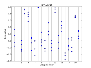
In statistics, the intraclass correlation, or the intraclass correlation coefficient (ICC), is a descriptive statistic that can be used when quantitative measurements are made on units that are organized into groups. It describes how strongly units in the same group resemble each other. While it is viewed as a type of correlation, unlike most other correlation measures, it operates on data structured as groups rather than data structured as paired observations.
A paired difference test, better known as a paired comparison, is a type of location test that is used when comparing two sets of paired measurements to assess whether their population means differ. A paired difference test is designed for situations where there is dependence between pairs of measurements. That applies in a within-subjects study design, i.e., in a study where the same set of subjects undergo both of the conditions being compared.
In survey research, the design effect is a number that shows how well a sample of people may represent a larger group of people for a specific measure of interest. This is important when the sample comes from a sampling method that is different than just picking people using a simple random sample.


