The likelihood function is the joint probability mass of observed data viewed as a function of the parameters of a statistical model. Intuitively, the likelihood function is the probability of observing data assuming is the actual parameter.
In statistics, the likelihood-ratio test assesses the goodness of fit of two competing statistical models, specifically one found by maximization over the entire parameter space and another found after imposing some constraint, based on the ratio of their likelihoods. If the constraint is supported by the observed data, the two likelihoods should not differ by more than sampling error. Thus the likelihood-ratio test tests whether this ratio is significantly different from one, or equivalently whether its natural logarithm is significantly different from zero.

In probability theory and statistics, the chi-squared distribution with degrees of freedom is the distribution of a sum of the squares of independent standard normal random variables. The chi-squared distribution is a special case of the gamma distribution and is one of the most widely used probability distributions in inferential statistics, notably in hypothesis testing and in construction of confidence intervals. This distribution is sometimes called the central chi-squared distribution, a special case of the more general noncentral chi-squared distribution.
In statistics, maximum likelihood estimation (MLE) is a method of estimating the parameters of an assumed probability distribution, given some observed data. This is achieved by maximizing a likelihood function so that, under the assumed statistical model, the observed data is most probable. The point in the parameter space that maximizes the likelihood function is called the maximum likelihood estimate. The logic of maximum likelihood is both intuitive and flexible, and as such the method has become a dominant means of statistical inference.

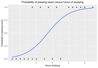
In statistics, the logistic model is a statistical model that models the log-odds of an event as a linear combination of one or more independent variables. In regression analysis, logistic regression is estimating the parameters of a logistic model. Formally, in binary logistic regression there is a single binary dependent variable, coded by an indicator variable, where the two values are labeled "0" and "1", while the independent variables can each be a binary variable or a continuous variable. The corresponding probability of the value labeled "1" can vary between 0 and 1, hence the labeling; the function that converts log-odds to probability is the logistic function, hence the name. The unit of measurement for the log-odds scale is called a logit, from logistic unit, hence the alternative names. See § Background and § Definition for formal mathematics, and § Example for a worked example.
Pearson's chi-squared test or Pearson's test is a statistical test applied to sets of categorical data to evaluate how likely it is that any observed difference between the sets arose by chance. It is the most widely used of many chi-squared tests – statistical procedures whose results are evaluated by reference to the chi-squared distribution. Its properties were first investigated by Karl Pearson in 1900. In contexts where it is important to improve a distinction between the test statistic and its distribution, names similar to Pearson χ-squared test or statistic are used.

An F-test is any statistical test used to compare the variances of two samples or the ratio of variances between multiple samples. The test statistic, random variable F, is used to determine if the tested data has an F-distribution under the true null hypothesis, and true customary assumptions about the error term (ε). It is most often used when comparing statistical models that have been fitted to a data set, in order to identify the model that best fits the population from which the data were sampled. Exact "F-tests" mainly arise when the models have been fitted to the data using least squares. The name was coined by George W. Snedecor, in honour of Ronald Fisher. Fisher initially developed the statistic as the variance ratio in the 1920s.
The Akaike information criterion (AIC) is an estimator of prediction error and thereby relative quality of statistical models for a given set of data. Given a collection of models for the data, AIC estimates the quality of each model, relative to each of the other models. Thus, AIC provides a means for model selection.
The Bayes factor is a ratio of two competing statistical models represented by their evidence, and is used to quantify the support for one model over the other. The models in question can have a common set of parameters, such as a null hypothesis and an alternative, but this is not necessary; for instance, it could also be a non-linear model compared to its linear approximation. The Bayes factor can be thought of as a Bayesian analog to the likelihood-ratio test, although it uses the integrated likelihood rather than the maximized likelihood. As such, both quantities only coincide under simple hypotheses. Also, in contrast with null hypothesis significance testing, Bayes factors support evaluation of evidence in favor of a null hypothesis, rather than only allowing the null to be rejected or not rejected.
In statistics, G-tests are likelihood-ratio or maximum likelihood statistical significance tests that are increasingly being used in situations where chi-squared tests were previously recommended.
In statistics, the score test assesses constraints on statistical parameters based on the gradient of the likelihood function—known as the score—evaluated at the hypothesized parameter value under the null hypothesis. Intuitively, if the restricted estimator is near the maximum of the likelihood function, the score should not differ from zero by more than sampling error. While the finite sample distributions of score tests are generally unknown, they have an asymptotic χ2-distribution under the null hypothesis as first proved by C. R. Rao in 1948, a fact that can be used to determine statistical significance.
In statistics, the Wald test assesses constraints on statistical parameters based on the weighted distance between the unrestricted estimate and its hypothesized value under the null hypothesis, where the weight is the precision of the estimate. Intuitively, the larger this weighted distance, the less likely it is that the constraint is true. While the finite sample distributions of Wald tests are generally unknown, it has an asymptotic χ2-distribution under the null hypothesis, a fact that can be used to determine statistical significance.
In statistics, Bartlett's test, named after Maurice Stevenson Bartlett, is used to test homoscedasticity, that is, if multiple samples are from populations with equal variances. Some statistical tests, such as the analysis of variance, assume that variances are equal across groups or samples, which can be checked with Bartlett's test.
In statistics, the Bayesian information criterion (BIC) or Schwarz information criterion is a criterion for model selection among a finite set of models; models with lower BIC are generally preferred. It is based, in part, on the likelihood function and it is closely related to the Akaike information criterion (AIC).
The goodness of fit of a statistical model describes how well it fits a set of observations. Measures of goodness of fit typically summarize the discrepancy between observed values and the values expected under the model in question. Such measures can be used in statistical hypothesis testing, e.g. to test for normality of residuals, to test whether two samples are drawn from identical distributions, or whether outcome frequencies follow a specified distribution. In the analysis of variance, one of the components into which the variance is partitioned may be a lack-of-fit sum of squares.
Omnibus tests are a kind of statistical test. They test whether the explained variance in a set of data is significantly greater than the unexplained variance, overall. One example is the F-test in the analysis of variance. There can be legitimate significant effects within a model even if the omnibus test is not significant. For instance, in a model with two independent variables, if only one variable exerts a significant effect on the dependent variable and the other does not, then the omnibus test may be non-significant. This fact does not affect the conclusions that may be drawn from the one significant variable. In order to test effects within an omnibus test, researchers often use contrasts.
In statistics, Wilks' lambda distribution, is a probability distribution used in multivariate hypothesis testing, especially with regard to the likelihood-ratio test and multivariate analysis of variance (MANOVA).
In statistics, the multinomial test is the test of the null hypothesis that the parameters of a multinomial distribution equal specified values; it is used for categorical data.
Log-linear analysis is a technique used in statistics to examine the relationship between more than two categorical variables. The technique is used for both hypothesis testing and model building. In both these uses, models are tested to find the most parsimonious model that best accounts for the variance in the observed frequencies.
In statistical hypothesis testing, the error exponent of a hypothesis testing procedure is the rate at which the probabilities of Type I and Type II decay exponentially with the size of the sample used in the test. For example, if the probability of error of a test decays as , where is the sample size, the error exponent is .


