Determination of equilibrium constants

Equilibrium constants are determined in order to quantify chemical equilibria. When an equilibrium constant K is expressed as a concentration quotient,

${\displaystyle K={\frac {\mathrm {[S]} ^{\sigma }\mathrm {[T]} ^{\tau }\cdots }{\mathrm {[A]} ^{\alpha }\mathrm {[B]} ^{\beta }\cdots }}}$

it is implied that the activity quotient is constant. For this assumption to be valid, equilibrium constants must be determined in a medium of relatively high ionic strength. Where this is not possible, consideration should be given to possible activity variation.

The equilibrium expression above is a function of the concentrations [A], [B] etc. of the chemical species in equilibrium. The equilibrium constant value can be determined if any one of these concentrations can be measured. The general procedure is that the concentration in question is measured for a series of solutions with known analytical concentrations of the reactants. Typically, a titration is performed with one or more reactants in the titration vessel and one or more reactants in the burette. Knowing the analytical concentrations of reactants initially in the reaction vessel and in the burette, all analytical concentrations can be derived as a function of the volume (or mass) of titrant added.

The equilibrium constants may be derived by best-fitting of the experimental data with a chemical model of the equilibrium system.

Experimental methods

There are four main experimental methods. For less commonly used methods, see Rossotti and Rossotti. ^[1] In all cases the range can be extended by using the competition method. An example of the application of this method can be found in palladium(II) cyanide.

Potentiometric measurements

A free concentration [A] or activity {A} of a species A is measured by means of an ion selective electrode such as the glass electrode. If the electrode is calibrated using activity standards it is assumed that the Nernst equation applies in the form

${\displaystyle E=E^{0}+{\frac {RT}{nF}}\ln \mathrm {\{A\}} }$

where E⁰ is the standard electrode potential. When buffer solutions of known pH are used for calibration the meter reading will be a pH.

${\displaystyle \mathrm {pH} ={\frac {nF}{RT}}\left(E^{0}-E\right)}$

At 298 K, 1 pH unit is approximately equal to 59 mV. ^[2]

When the electrode is calibrated with solutions of known concentration, by means of a strong acid–strong base titration, for example, a modified Nernst equation is assumed.

${\displaystyle E=E^{0}+s\log _{10}\mathrm {[A]} }$

where s is an empirical slope factor. A solution of known hydrogen ion concentration may be prepared by standardization of a strong acid against borax. Constant-boiling hydrochloric acid may also be used as a primary standard for hydrogen ion concentration.

Range and limitations

The most widely used electrode is the glass electrode, which is selective for the hydrogen ion. This is suitable for all acid–base equilibria. log₁₀β values between about 2 and 11 can be measured directly by potentiometric titration using a glass electrode. This enormous range of stability constant values (ca. 100 to 10¹¹) is possible because of the logarithmic response of the electrode. The limitations arise because the Nernst equation breaks down at very low or very high pH.

When a glass electrode is used to obtain the measurements on which the calculated equilibrium constants depend, the precision of the calculated parameters is limited by secondary effects such as variation of liquid junction potentials in the electrode. In practice it is virtually impossible to obtain a precision for log β better than ±0.001.

Spectrophotometric measurements

Absorbance

It is assumed that the Beer–Lambert law applies.

${\displaystyle A=l\sum {\varepsilon c}}$

where l is the optical path length, ε is a molar absorbance at unit path length and c is a concentration. More than one of the species may contribute to the absorbance. In principle absorbance may be measured at one wavelength only, but in present-day practice it is common to record complete spectra.

Range and limitations

An upper limit on log₁₀β of 4 is usually quoted, corresponding to the precision of the measurements, but it also depends on how intense the effect is. Spectra of contributing species should be clearly distinct from each other

Fluorescence (luminescence) intensity

It is assumed that the scattered light intensity is a linear function of species’ concentrations.

${\displaystyle I=\sum \varphi c}$

where φ is a proportionality constant.

Range and limitations

The magnitude of the constant φ may be higher than the value of the molar extinction coefficient, ε, for a species. When this is so, the detection limit for that species will be lower. At high solute concentrations, fluorescence intensity becomes non-linear with respect to concentration due to self-absorption of the scattered radiation.

NMR chemical shift measurements

Chemical exchange is assumed to be rapid on the NMR time-scale. An individual chemical shift δ is the mole-fraction-weighted average of the shifts δ of nuclei in contributing species.

${\displaystyle {\bar {\delta }}={\frac {\sum x_{i}\delta _{i}}{\sum x_{i}}}}$

Example: the pK_a of the hydroxyl group in citric acid has been determined from ¹³C chemical shift data to be 14.4. Neither potentiometry nor ultraviolet–visible spectroscopy could be used for this determination. ^[3]

Range and limitations

Limited precision of chemical shift measurements also puts an upper limit of about 4 on log₁₀β. Limited to diamagnetic systems. ¹H NMR cannot be used with solutions of compounds in ¹H₂O.

Calorimetric measurements

Simultaneous measurement of K and ΔH for 1:1 adducts is routinely carried out using isothermal titration calorimetry. Extension to more complex systems is limited by the availability of suitable software.

Range and limitations

Insufficient evidence is currently available.

The competition method

The competition method may be used when a stability constant value is too large to be determined by a direct method. It was first used by Schwarzenbach in the determination of the stability constants of complexes of EDTA with metal ions.

For simplicity consider the determination of the stability constant ${\displaystyle K_{AB}}$ of a binary complex, AB, of a reagent A with another reagent B.

${\displaystyle K_{AB}={\frac {[AB]}{[A][B]}}}$

where the [X] represents the concentration, at equilibrium, of a species X in a solution of given composition.

A ligand C is chosen which forms a weaker complex with A The stability constant, K_AC, is small enough to be determined by a direct method. For example, in the case of EDTA complexes A is a metal ion and C may be a polyamine such as diethylenetriamine.

${\displaystyle K_{AC}={\frac {[AC]}{[A][C]}}}$

The stability constant, K for the competition reaction

${\displaystyle AC+B\leftrightharpoons AB+C}$

can be expressed as

${\displaystyle K={\frac {[AB][C]}{[AC][B]}}}$

It follows that

${\displaystyle K_{AB}=K\times K_{AC}}$

where K is the stability constant for the competition reaction. Thus, the value of the stability constant ${\displaystyle K_{AB}}$ may be derived from the experimentally determined values of K and ${\displaystyle K_{AC}}$ .

Computational methods

It is assumed that the collected experimental data comprise a set of data points. At each ith data point, the analytical concentrations of the reactants, T_A(i), T_B(i) etc. are known along with a measured quantity, y_i, that depends on one or more of these analytical concentrations. A general computational procedure has four main components:

1. Definition of a chemical model of the equilibria
2. Calculation of the concentrations of all the chemical species in each solution
3. Refinement of the equilibrium constants
4. Model selection

The value of the equilibrium constant for the formation of a 1:1 complex, such as a host-guest species, may be calculated with a dedicated spreadsheet application, Bindfit: ^[4] In this case step 2 can be performed with a non-iterative procedure and the pre-programmed routine Solver can be used for step 3.

The chemical model

The chemical model consists of a set of chemical species present in solution, both the reactants added to the reaction mixture and the complex species formed from them. Denoting the reactants by A, B..., each complex species is specified by the stoichiometric coefficients that relate the particular combination of reactants forming them.

${\displaystyle {\ce {{{\mathit {p}}A}+{\mathit {q}}B\cdots <=>A_{\mathit {p}}B_{\mathit {q}}\cdots }}}$: ${\displaystyle \beta _{pq\cdots }={\frac {[{\ce {A}}_{p}{\ce {B}}_{q}\cdots ]}{[{\ce {A}}]^{p}[{\ce {B}}]^{q}\cdots }}}$

When using general-purpose computer programs, it is usual to use cumulative association constants, as shown above. Electrical charges are not shown in general expressions such as this and are often omitted from specific expressions, for simplicity of notation. In fact, electrical charges have no bearing on the equilibrium processes other that there being a requirement for overall electrical neutrality in all systems.

With aqueous solutions the concentrations of proton (hydronium ion) and hydroxide ion are constrained by the self-dissociation of water.

${\displaystyle {\ce {H2O <=> H+ + OH-}}}$: ${\displaystyle K_{\mathrm {W} }^{'}={\frac {[H^{+}][OH^{-}]}{[H_{2}O]}}}$

With dilute solutions the concentration of water is assumed constant, so the equilibrium expression is written in the form of the ionic product of water.

${\displaystyle K_{\mathrm {W} }={\ce {[H+]}}[{\ce {OH-}}]\,}$

When both H⁺ and OH⁻ must be considered as reactants, one of them is eliminated from the model by specifying that its concentration be derived from the concentration of the other. Usually the concentration of the hydroxide ion is given by

${\displaystyle [{\ce {OH-}}]={\frac {K_{{\ce {W}}}}{[{\ce {H+}}]}}\,}$

In this case the equilibrium constant for the formation of hydroxide has the stoichiometric coefficients −1 in regard to the proton and zero for the other reactants. This has important implications for all protonation equilibria in aqueous solution and for hydrolysis constants in particular.

It is quite usual to omit from the model those species whose concentrations are considered negligible. For example, it is usually assumed then there is no interaction between the reactants and/or complexes and the electrolyte used to maintain constant ionic strength or the buffer used to maintain constant pH. These assumptions may or may not be justified. Also, it is implicitly assumed that there are no other complex species present. When complexes are wrongly ignored a systematic error is introduced into the calculations.

Equilibrium constant values are usually estimated initially by reference to data sources.

Speciation calculations

A speciation calculation is one in which concentrations of all the species in an equilibrium system are calculated, knowing the analytical concentrations, T_A, T_B etc. of the reactants A, B etc. This means solving a set of nonlinear equations of mass-balance

${\displaystyle {\begin{aligned}{\ce {T_{A}}}&=[{\ce {A}}]+\sum _{1,nk}p\beta _{pq\cdots }[{\ce {A}}]^{p}[{\ce {B}}]^{q}\cdots \\{\ce {T_{B}}}&=[{\ce {B}}]+\sum _{1,nk}q\beta _{pq\cdots }[{\ce {A}}]^{p}[{\ce {B}}]^{q}\cdots \\etc.\end{aligned}}}$

for the free concentrations [A], [B] etc. When the pH (or equivalent e.m.f., E).is measured, the free concentration of hydrogen ions, [H], is obtained from the measured value as

${\displaystyle [\mathrm {H} ]=10^{-\mathrm {pH} }}$ or ${\displaystyle [\mathrm {H} ]=e^{\mathrm {{-{\frac {nF}{RT}}}(E-E^{0})} }}$

and only the free concentrations of the other reactants are calculated. The concentrations of the complexes are derived from the free concentrations via the chemical model.

Some authors ^{[5] [6]} include the free reactant terms in the sums by declaring identity (unit) β constants for which the stoichiometric coefficients are 1 for the reactant concerned and zero for all other reactants. For example, with 2 reagents, the mass-balance equations assume the simpler form.

${\displaystyle {\begin{aligned}T_{\ce {A}}&=\sum _{0,nk}p\beta _{pq}[{\ce {A}}]^{p}[{\ce {B}}]^{q}\\[4pt]T_{\ce {B}}&=\sum _{0,nk}q\beta _{pq}[{\ce {A}}]^{p}[{\ce {B}}]^{q}\\\end{aligned}}}$

${\displaystyle \beta _{10}=\beta _{01}=1}$

In this manner, all chemical species, including the free reactants, are treated in the same way, having been formed from the combination of reactants that is specified by the stoichiometric coefficients.

In a titration system the analytical concentrations of the reactants at each titration point are obtained from the initial conditions, the burette concentrations and volumes. The analytical (total) concentration of a reactant R at the ith titration point is given by

${\displaystyle T_{{\ce {R}}}={\frac {{\ce {R}}_{0}+v_{i}{\ce {[R]}}}{v_{0}+v_{i}}}}$

where R₀ is the initial amount of R in the titration vessel, v₀ is the initial volume, [R] is the concentration of R in the burette and v_i is the volume added. The burette concentration of a reactant not present in the burette is taken to be zero.

In general, solving these nonlinear equations presents a formidable challenge because of the huge range over which the free concentrations may vary. At the beginning, values for the free concentrations must be estimated. Then, these values are refined, usually by means of Newton–Raphson iterations. The logarithms of the free concentrations may be refined rather than the free concentrations themselves. Refinement of the logarithms of the free concentrations has the added advantage of automatically imposing a non-negativity constraint on the free concentrations. Once the free reactant concentrations have been calculated, the concentrations of the complexes are derived from them and the equilibrium constants.

Note that the free reactant concentrations can be regarded as implicit parameters in the equilibrium constant refinement process. In that context the values of the free concentrations are constrained by forcing the conditions of mass-balance to apply at all stages of the process.

Equilibrium constant refinement

The objective of the refinement process is to find equilibrium constant values that give the best fit to the experimental data. This is usually achieved by minimising an objective function, U, by the method of non-linear least-squares. First the residuals are defined as

${\displaystyle r_{i}=y_{i}^{\text{obs}}-y_{i}^{\text{calc}}}$

Then the most general objective function is given by

${\displaystyle U=\sum _{i}\sum _{j}r_{i}W_{ij}r_{j}\,}$

The matrix of weights, W, should be, ideally, the inverse of the variance-covariance matrix of the observations. It is rare for this to be known. However, when it is, the expectation value of U is one, which means that the data are fitted within experimental error. Most often only the diagonal elements are known, in which case the objective function simplifies to

${\displaystyle U=\sum _{i}W_{ii}r_{i}^{2}}$

with W_ij = 0 when j ≠ i. Unit weights, W_ii = 1, are often used but, in that case, the expectation value of U is the root mean square of the experimental errors.

The minimization may be performed using the Gauss–Newton method. Firstly the objective function is linearised by approximating it as a first-order Taylor series expansion about an initial parameter set, p.

${\displaystyle U=U^{0}+\sum _{i}{\frac {\partial U}{\partial p_{i}}}\delta p_{i}}$

The increments δp_i are added to the corresponding initial parameters such that U is less than U⁰. At the minimum the derivatives ⁠∂U/∂p_i⁠, which are simply related to the elements of the Jacobian matrix, J

${\displaystyle J_{jk}={\frac {\partial y_{j}^{\mathrm {calc} }}{\partial p_{k}}}}$

where p_k is the kth parameter of the refinement, are equal to zero. One or more equilibrium constants may be parameters of the refinement. However, the measured quantities (see above) represented by y are not expressed in terms of the equilibrium constants, but in terms of the species concentrations, which are implicit functions of these parameters. Therefore, the Jacobian elements must be obtained using implicit differentiation.

The parameter increments δp are calculated by solving the normal equations, derived from the conditions that ⁠∂U/∂p⁠ = 0 at the minimum.

${\displaystyle {\left(J^{\mathrm {T} }WJ\right)\delta p=J^{\mathrm {T} }Wr}}$

The increments δp are added iteratively to the parameters

${\displaystyle \mathbf {p} ^{n+1}=\mathbf {p} ^{n}+\delta \mathbf {p} }$

where n is an iteration number. The species concentrations and y^calc values are recalculated at every data point. The iterations are continued until no significant reduction in U is achieved, that is, until a convergence criterion is satisfied. If, however, the updated parameters do not result in a decrease of the objective function, that is, if divergence occurs, the increment calculation must be modified. The simplest modification is to use a fraction, f, of calculated increment, so-called shift-cutting.

${\displaystyle \mathbf {p} ^{n+1}=\mathbf {p} ^{n}+f\mathbf {\delta p} }$

In this case, the direction of the shift vector, δp, is unchanged. With the more powerful Levenberg–Marquardt algorithm, on the other hand, the shift vector is rotated towards the direction of steepest descent, by modifying the normal equations,

${\displaystyle \mathbf {\left(J^{\mathrm {T} }WJ+\lambda I\right)\delta p=J^{\mathrm {T} }Wr} }$

where λ is the Marquardt parameter and I is an identity matrix. Other methods of handling divergence have been proposed. ^[6]

A particular issue arises with NMR and spectrophotometric data. For the latter, the observed quantity is absorbance, A, and the Beer–Lambert law can be written as

${\displaystyle A_{\lambda }=l\sum (\varepsilon _{pq..})_{\lambda }c_{pq..}}$

It can be seen that, assuming that the concentrations, c, are known, that absorbance, A, at a given wavelength, ${\displaystyle \lambda }$, and path length ${\displaystyle l}$, is a linear function of the molar absorptivities, ε. With 1 cm path-length, in matrix notation

${\displaystyle \mathbf {A} ={\boldsymbol {\varepsilon }}\mathbf {C} \,}$

There are two approaches to the calculation of the unknown molar absorptivities

(1) The ε values are considered parameters of the minimization and the Jacobian is constructed on that basis. However, the ε values themselves are calculated at each step of the refinement by linear least-squares:

${\displaystyle {\boldsymbol {\varepsilon }}=\mathbf {\left(C^{\mathrm {T} }C\right)^{-1}C^{\mathrm {T} }A} }$

using the refined values of the equilibrium constants to obtain the speciation. The matrix

${\displaystyle \mathbf {\left(C^{T}C\right)^{-1}C^{T}} }$

is an example of a pseudo-inverse.

Golub and Pereyra ^[7] showed how the pseudo-inverse can be differentiated so that parameter increments for both molar absorptivities and equilibrium constants can be calculated by solving the normal equations.

(2) The Beer–Lambert law is written as

${\displaystyle \mathbf {\boldsymbol {\varepsilon }} _{\lambda }=\mathbf {A} _{\lambda }^{-1}\mathbf {C} \,}$

The unknown molar absorbances of all "coloured" species are found by using the non-iterative method of linear least-squares, one wavelength at a time. The calculations are performed once every refinement cycle, using the stability constant values obtaining at that refinement cycle to calculate species' concentration values in the matrix ${\displaystyle \mathbf {C} }$.

Parameter errors and correlation

In the region close to the minimum of the objective function, U, the system approximates to a linear least-squares system, for which

${\displaystyle \mathbf {p=\left(J^{\mathrm {T} }WJ\right)^{-1}J^{\mathrm {T} }Wy^{\mathrm {obs} }} }$

Therefore, the parameter values are (approximately) linear combinations of the observed data values and the errors on the parameters, p, can be obtained by error propagation from the observations, y^obs, using the linear formula. Let the variance-covariance matrix for the observations be denoted by Σ^y and that of the parameters by Σ^p. Then,

${\displaystyle \mathbf {\Sigma ^{p}=\left(J^{\mathrm {T} }WJ\right)^{-1}J^{\mathrm {T} }W\Sigma ^{y}W^{\mathrm {T} }J(J^{\mathrm {T} }WJ)^{-1}} }$

When W = (Σ^y)⁻¹, this simplifies to

${\displaystyle \mathbf {\Sigma ^{p}=\left(J^{\mathrm {T} }WJ\right)^{-1}} }$

In most cases the errors on the observations are un-correlated, so that Σ^y is diagonal. If so, each weight should be the reciprocal of the variance of the corresponding observation. For example, in a potentiometric titration, the weight at a titration point, k, can be given by

${\displaystyle W_{k}={\frac {1}{\sigma _{E}^{2}+\left({\frac {\partial E}{\partial v}}\right)_{k}^{2}\sigma _{v}^{2}}}}$

where σ_E is the error in electrode potential or pH, (⁠∂E/∂v⁠)
_^k is the slope of the titration curve and σ_v is the error on added volume.

When unit weights are used (W = I, p = (J^TJ)⁻¹J^Ty) it is implied that the experimental errors are uncorrelated and all equal: Σ^y = σ²I, where σ² is known as the variance of an observation of unit weight, and I is an identity matrix. In this case σ² is approximated by

${\displaystyle \sigma ^{2}={\frac {U}{n_{\mathrm {d} }-n_{\mathrm {p} }}}}$

where U is the minimum value of the objective function and n_d and n_p are the number of data and parameters, respectively.

${\displaystyle \mathbf {\Sigma ^{p}} ={\frac {U}{n_{\mathrm {d} }-n_{\mathrm {p} }}}\left(\mathbf {J} ^{\mathrm {T} }\mathbf {J} \right)^{-1}}$

In all cases, the variance of the parameter p_i is given by Σ^p
_ii and the covariance between parameters p_i and p_j is given by Σ^p
_ij. Standard deviation is the square root of variance. These error estimates reflect only random errors in the measurements. The true uncertainty in the parameters is larger due to the presence of systematic errors—which, by definition, cannot be quantified.

Note that even though the observations may be uncorrelated, the parameters are always correlated.

Derived constants

When cumulative constants have been refined it is often useful to derive stepwise constants from them. The general procedure is to write down the defining expressions for all the constants involved and then to equate concentrations. For example, suppose that one wishes to derive the pKa for removing one proton from a tribasic acid, LH₃, such as citric acid.

${\displaystyle {\begin{aligned}{\ce {L^3-}}+{\ce {H+ <=>}}\ {\ce {LH^2-}}&:\ [{\ce {LH^2-}}]=\beta _{11}[{\ce {L^3-}}][{\ce {H+}}]\\{\ce {L^3-}}+{\ce {2H+ <=>}}\ {\ce {LH2^-}}&:\ [{\ce {LH2^-}}]=\beta _{12}[{\ce {L^3-}}][{\ce {H+}}]^{2}\\{\ce {L^3-}}+{\ce {3H+ <=>}}\ {\ce {LH3}}&:\ [{\ce {LH3}}]=\beta _{13}[{\ce {L^3-}}][{\ce {H+}}]^{3}\end{aligned}}}$

The stepwise association constant for formation of LH₃ is given by

${\displaystyle {\ce {{LH2^{-}}+H+<=>LH3\$ ;\quad \ [LH3]}}=K[{\ce {LH2^{-}}}][{\ce {H+}}]}

Substitute the expressions for the concentrations of LH₃ and LH⁻
₂ into this equation

${\displaystyle \beta _{13}[{\ce {L^3-}}][{\ce {H+}}]^{3}=K\beta _{12}[{\ce {L^3-}}][{\ce {H+}}]^{2}[{\ce {H+}}]}$

whence

${\displaystyle \beta _{13}=K\beta _{12};K={\frac {\beta _{13}}{\beta _{12}}}\,}$

and since pK_a = −log₁₀⁠1/K⁠ its value is given by

${\displaystyle {\ce {p}}K_{{\ce {a1}}}=\log _{10}\beta _{13}-\log _{10}\beta _{12}\,}$

${\displaystyle {\ce {p}}K_{{\ce {a2}}}=\log _{10}\beta _{12}-\log _{10}\beta _{11}\,}$

${\displaystyle {\ce {p}}K_{{\ce {a3}}}=\log _{10}\beta _{11}\,}$

Note the reverse numbering for pK and log β. When calculating the error on the stepwise constant, the fact that the cumulative constants are correlated must accounted for. By error propagation

${\displaystyle \sigma _{K}^{2}=\sigma _{\beta _{12}}^{2}+\sigma _{\beta _{13}}^{2}-2\sigma _{\beta _{12}}\sigma _{\beta _{13}}\rho _{12,13}\,}$

and

${\displaystyle \sigma _{\log _{10}K}={\frac {\sigma _{K}}{K}}}$

Model selection

Once a refinement has been completed the results should be checked to verify that the chosen model is acceptable. generally speaking, a model is acceptable when the data are fitted within experimental error, but there is no single criterion to use to make the judgement. The following should be considered.

The objective function

When the weights have been correctly derived from estimates of experimental error, the expectation value of ⁠U/n_d − n_p⁠ is 1. ^[8] It is therefore very useful to estimate experimental errors and derive some reasonable weights from them as this is an absolute indicator of the goodness of fit.

When unit weights are used, it is implied that all observations have the same variance. ⁠U/n_d − n_p⁠ is expected to be equal to that variance.

Parameter errors

One would want the errors on the stability constants to be roughly commensurate with experimental error. For example, with pH titration data, if pH is measured to 2 decimal places, the errors of log₁₀β should not be much larger than 0.01. In exploratory work where the nature of the species present is not known in advance, several different chemical models may be tested and compared. There will be models where the uncertainties in the best estimate of an equilibrium constant may be somewhat or even significantly larger than σ_pH, especially with those constants governing the formation of comparatively minor species, but the decision as to how large is acceptable remains subjective. The decision process as to whether or not to include comparatively uncertain equilibria in a model, and for the comparison of competing models in general, can be made objective and has been outlined by Hamilton. ^[8]

Distribution of residuals

At the minimum in U the system can be approximated to a linear one, the residuals in the case of unit weights are related to the observations by

${\displaystyle \mathbf {r=y^{\mathrm {obs} }-J\left(J^{\mathrm {T} }T\right)^{-1}J^{\mathrm {T} }y^{\mathrm {obs} }} }$

The symmetric, idempotent matrix J(J^TT)⁻¹J is known in the statistics literature as the hat matrix, H. Thus,

${\displaystyle \mathbf {r=\left(I-H\right)y^{\mathrm {obs} }} }$

and

${\displaystyle \mathbf {M^{r}=\left(I-H\right)M^{y}\left(I-H\right)} }$

where I is an identity matrix and M^r and M^y are the variance-covariance matrices of the residuals and observations, respectively. This shows that even though the observations may be uncorrelated, the residuals are always correlated.

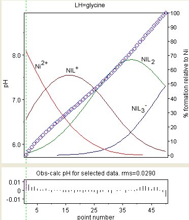
The diagram at the right shows the result of a refinement of the stability constants of Ni(Gly)⁺, Ni(Gly)₂ and Ni(Gly)⁻
₃ (where GlyH = glycine). The observed values are shown a blue diamonds and the species concentrations, as a percentage of the total nickel, are superimposed. The residuals are shown in the lower box. The residuals are not distributed as randomly as would be expected. This is due to the variation of liquid junction potentials and other effects at the glass/liquid interfaces. Those effects are very slow compared to the rate at which equilibrium is established.

Physical constraints

Some physical constraints are usually incorporated in the calculations. For example, all the concentrations of free reactants and species must have positive values and association constants must have positive values.

With spectrophotometric data the calculated molar absorptivity (or emissivity) values should all be positive. Most computer programs do not impose this constraint on the calculations.

Chemical constraints

When determining the stability constants of metal-ligand complexes, it is common practice to fix ligand protonation constants at values that have been determined using data obtained from metal-free solutions. Hydrolysis constants of metal ions are usually fixed at values which were obtained using ligand-free solutions. When determining the stability constants for ternary complexes, M_pA_qB_r it is common practice the fix the values for the corresponding binary complexes M_p′A_q′ and M_p′′B_q′′, at values which have been determined in separate experiments. Use of such constraints reduces the number of parameters to be determined, but may result in the calculated errors on refined stability constant values being under-estimated.

Other models

If the model is not acceptable, a variety of other models should be examined to find one that best fits the experimental data, within experimental error. The main difficulty is with the so-called minor species. These are species whose concentration is so low that the effect on the measured quantity is at or below the level of error in the experimental measurement. The constant for a minor species may prove impossible to determine if there is no means to increase the concentration of the species. .

Thermodynamic principles of host–guest interactions

The thermodynamics of the host- guest interaction can be assessed by NMR spectroscopy, UV/visible spectroscopy, and isothermal titration calorimetry. ^[9] Quantitative analysis of binding constant values provides useful thermodynamic information. ^[10]

An association constant, ${\displaystyle K_{a}^{\ominus }}$ can be defined by the expression

${\displaystyle K_{a}^{\ominus }={\frac {\{HG\}}{\{H\}\{G\}}}={\frac {[HG]}{[H][G]}}\times \Gamma }$

where {HG} is the thermodynamic activity of the complex at equilibrium. {H} represents the activity of the host and {G} the activity of the guest. The quantities ${\displaystyle [HG]}$, ${\displaystyle [H]}$ and ${\displaystyle [G]}$ are the corresponding concentrations and ${\displaystyle \Gamma }$ is a quotient of activity coefficients.

In practice the equilibrium constant is usually defined in terms of concentrations.

${\displaystyle K_{a}={\frac {[HG]}{[H][G]}}}$

When this definition is used, it is implied that the quotient of activity coefficients has a numerical value of one. It then appears that the equilibrium constant, ${\displaystyle K_{A}}$ has the dimension 1/concentration, but that cannot be true since the standard Gibbs free energy change, ${\displaystyle \Delta G^{\ominus }}$ is proportional to the logarithm of ${\displaystyle K_{A}}$.

${\displaystyle \Delta G^{\ominus }=-RT\ln {K_{A}^{\ominus }}}$

This apparent paradox is resolved when the dimension of ${\displaystyle \Gamma }$ is defined to be the reciprocal of the dimension of the quotient of concentrations. The implication is that ${\displaystyle \Gamma }$ is regarded as having a constant value under all relevant experimental conditions. Nevertheless it is common practice to attach a dimension, such as millimole per litre or micromole per litre, to a value of K that has been determined experimentally.

A Large ${\displaystyle K_{a}}$ value indicates that host and guest molecules interact strongly to form the host–guest complex.

Determination of binding constant values and kinetic constant

Main article: Determination of equilibrium constants

Simple host–guest complexation

When the host and guest molecules combine to form a single complex, the equilibrium is represented as

${\displaystyle H+G\leftrightharpoons HG}$

and the equilibrium constant, K, is defined as

${\displaystyle K={\frac {[HG]}{[H][G]}}}$

where [X] denotes the concentration of a chemical species X (all activity coefficients are assumed to have a numerical values of 1). The mass-balance equations, at any data point,

${\displaystyle T_{H}=[H]+K[H][G]}$

${\displaystyle T_{G}=[G]+K[H][G]}$

where ${\displaystyle T_{G}}$ and ${\displaystyle T_{H}}$ represent the total concentrations, of host and guest, can be reduced to a single quadratic equation in, say, [G] and so can be solved analytically for any given value of K. The concentrations [H] and [HG] can then derived.

${\displaystyle [H]=T_{H}-T_{G}+[G]}$

${\displaystyle [HG]=K[H][G]}$

The next step in the calculation is to calculate the value, ${\displaystyle X_{i}^{calc}}$, of a quantity corresponding to the quantity observed ${\displaystyle X_{i}^{obs}}$. Then, a sum of squares, U, over all data points, np, can be defined as

${\displaystyle U=\sum _{i=1,np}(X_{i}^{obs}-X_{i}^{calc})^{2}}$

and this can be minimized with respect to the stability constant value, K, and a parameter such the chemical shift of the species HG (nmr data) or its molar absorbency (uv/vis data). The minimization can be performed in a spreadsheet application such as EXCEL by using the in-built SOLVER utility.

This procedure is applicable to 1:1 adducts.

General complexation reaction

For each equilibrium involving a host, H, and a guest G

${\displaystyle pH+qG\leftrightharpoons H_{p}G_{q}}$

the equilibrium constant, ${\displaystyle \beta _{pq}}$, is defined as

${\displaystyle \beta _{pq}={\frac {[H_{p}G_{q}]}{[H]^{p}[G]^{q}}}}$

The values of the free concentrations, ${\displaystyle [H]}$ and ${\displaystyle [G]}$ are obtained by solving the equations of mass balance with known or estimated values for the stability constants.

${\displaystyle T_{H}=[H]+\sum p\beta _{pq}[H]^{p}[G]^{q}}$

${\displaystyle T_{G}=[G]+\sum q\beta _{pq}[H]^{p}[G]^{q}}$

Then, the concentrations of each complex species may also be calculated as ${\displaystyle [H_{p}G_{q}]=\beta _{pq}[H]^{p}[G]^{q}}$. The relationship between a species' concentration and the measured quantity is specific for the measurement technique, as indicated in each section above. Using this relationship, the set of parameters, the stability constant values and values of properties such as molar absorptivity or specified chemical shifts, may be refined by a non-linear least-squares refinement process. For a more detailed exposition of the theory see Determination of equilibrium constants. Some dedicated computer programs are listed at Implementations.

Cooperativity

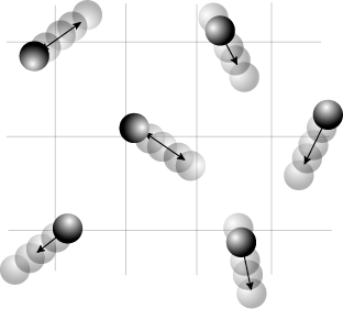
In cooperativity, the initial ligand binding affects the host's affinity for subsequent ligands. In positive cooperativity, the first binding event enhances the affinity of the host for another ligand. Examples of positive and negative cooperativity are hemoglobin and aspartate receptor, respectively. ^[11]

General Host–Guest Binding. (1.) Guest A binding (2.) Guest B binding. (3.) Positive Cooperativity Guest A–B binding. (4.) Negative Cooperativity Guest A–B binding

The thermodynamic properties of cooperativity have been studied in order to define mathematical parameters that distinguish positive or negative cooperativity. The traditional Gibbs free energy equation states: ${\displaystyle \Delta G=\Delta H-T\Delta S\ }$. However, to quantify cooperativity in a host–guest system, the binding energy needs to be considered. The schematic on the right shows the binding of A, binding of B, positive cooperative binding of A–B, and lastly, negative cooperative binding of A–B. Therefore, an alternate form of the Gibbs free energy equation would be

${\displaystyle \Delta G_{S}^{\circ }=\Delta G_{A}^{\circ }+\Delta G_{B}^{\circ }-\Delta G_{AB}^{\circ }}$

${\displaystyle \Delta H_{S}^{\circ }=\Delta H_{A}^{\circ }+\Delta H_{B}^{\circ }-\Delta H_{AB}^{\circ }}$

${\displaystyle \ T\Delta G_{S}^{\circ }=T\Delta H_{A}^{\circ }+T\Delta H_{B}^{\circ }-T\Delta S_{AB}^{\circ }}$

where:

${\displaystyle \Delta G_{A}^{\circ }}$ = free energy of binding A

${\displaystyle \Delta G_{B}^{\circ }}$ = free energy of binding B

${\displaystyle \Delta G_{S}^{\circ }}$ = free energy of binding for A and B tethered

${\displaystyle \Delta G_{AB}^{\circ }}$ = sum of the free energies of binding

It is considered that if ${\displaystyle \Delta G_{S}^{\circ }}$ more than the sum of ${\displaystyle \Delta G_{A}^{\circ }}$ and ${\displaystyle \Delta G_{B}^{\circ }}$, it is positively cooperative. If ${\displaystyle \Delta G_{S}^{\circ }}$ is less, then it is negatively cooperative. ^[12] Host–guest chemistry is not limited to receptor-lingand interactions. It is also demonstrated in ion-pairing systems. Such interactions are studied in an aqueous media utilizing synthetic organometallic hosts and organic guest molecules. For example, a poly-cationic receptor containing copper (the host) is coordinated with molecules such as tetracarboxylates, tricarballate, aspartate, and acetate (the guests). This study illustrates that entropy rather than enthalpy determines the binding energy of the system leading to negative cooperativity. The large change in entropy originates from the displacement of solvent molecules surrounding the ligand and the receptor. When multiple acetates bind to the receptor, it releases more water molecules to the environment than a tetracarboxylate. This led to a decrease in free energy implying that the system is cooperating negatively. ^[13] In a similar study, utilizing guanidinium and Cu(II) and polycarboxylate guests, it is demonstrated that positive cooperatively is largely determined by enthalpy. ^[14] In addition to thermodynamic studies, host–guest chemistry also has biological applications.

Implementations

Some simple systems are amenable to spreadsheet calculations. ^{[4] [15]}

A large number of general-purpose computer programs for equilibrium constant calculation have been published. See ^[16] for a bibliography. The most frequently used programs are:

• Potentiometric data: Hyperquad, BEST ^[17] PSEQUAD, ^[18] ReactLab pH PRO
• Spectrophotometric data:HypSpec, SQUAD, ^[18] Specfit, ^[19] ReactLab EQUILIBRIA
• NMR data HypNMR, EQNMR Archived 2019-07-14 at the Wayback Machine
• Calorimetric data HypΔH. Affinimeter
  Commercial Isothermal titration calorimeters are usually supplied with software with which an equilibrium constant and standard formation enthalpy for the formation of a 1:1 adduct can be obtained. Some software for handling more complex equilibria may also be supplied.

References

1. Rossotti, F. J. C.; Rossotti, H. (1961). The Determination of Stability Constants. McGraw-Hill.
2. "Definitions of pH scales, standard reference values, measurement of pH, and related terminology" (PDF). Pure Appl. Chem. 57: 531–542. 1985. doi:10.1351/pac198557030531. S2CID   14182410.
3. Silva, Andre M. N.; Kong, Xiaole; Hider, Robert C. (2009). "Determination of the pK_a value of the hydroxyl group in the α-hydroxycarboxylates citrate, malate and lactate by ¹³C NMR: implications for metal coordination in biological systems". Biometals. 22 (5): 771–778. doi:10.1007/s10534-009-9224-5. PMID   19288211. S2CID   11615864.
4. Hibbert, D.B.; Thordarson, P. (2017). "The death of the Job plot, transparency, open science and online tools, uncertainty estimation methods and other developments in supramolecular chemistry data analysis". Chemical Communications. 52 (87): 12792–12805. doi: 10.1039/c6cc03888c . PMID   27779264.
5. Motekaitis, R. J.; Martell, A. E. (1982). "BEST — A new program for rigorous calculation of equilibrium parameters of complex multicomponent systems". Can. J. Chem. 60 (19): 2403–2409. doi:10.1139/v82-347.
6. Potvin, P. G. (1990). "Modelling complex solution equilibria. I. Fast, worry-free least-squares refinement of equilibrium constants". Can. J. Chem. 68 (12): 2198–2207. doi: 10.1139/v90-337 .
7. Golub, G. H.; Pereyra, V. (1973). "The Differentiation of Pseudo-Inverses and Nonlinear Least Squares Problems Whose Variables Separate". SIAM J. Numer. Anal. 10 (2): 413–432. Bibcode:1973SJNA...10..413G. doi:10.1137/0710036.
8. Hamilton, W. C. (1964). Statistics in Physical Science . New York, NY: Ronald Press.
9. Piñeiro, Á.; Banquy, X.; Pérez-Casas, S.; Tovar, É.; García, A.; Villa, A.; Amigo, A.; Mark, A. E.; Costas, M. (2007). "On the Characterization of Host–Guest Complexes: Surface Tension, Calorimetry, and Molecular Dynamics of Cyclodextrins with a Non-ionic Surfactant". Journal of Physical Chemistry B. 111 (17): 4383–92. doi:10.1021/jp0688815. PMID   17428087.
11. Koshland, D (1996). "The structural basis of negative cooperativity: receptors and enzymes". Current Opinion in Structural Biology . 6 (6): 757–761. doi:10.1016/S0959-440X(96)80004-2. PMID   8994875.
12. Jencks, W. P. (1981). "On the attribution and additivity of binding energies". Proceedings of the National Academy of Sciences, USA . 78 (7): 4046–4050. Bibcode:1981PNAS...78.4046J. doi: 10.1073/pnas.78.7.4046 . PMC   319722 . PMID   16593049.
13. Dobrzanska, L; Lloyd, G; Esterhuysen, C; Barbour, L (2003). "Studies into the Thermodynamic Origin of Negative Cooperativity in Ion-Pairing Molecular Recognition". Journal of the American Chemical Society . 125 (36): 10963–10970. doi:10.1021/ja030265o. PMID   12952478.
14. Hughes, A.; Anslyn, E (2007). "A cationic host displaying positive cooperativity in water". Proceedings of the National Academy of Sciences, USA . 104 (16): 6538–6543. Bibcode:2007PNAS..104.6538H. doi: 10.1073/pnas.0609144104 . PMC   1871821 . PMID   17420472.
15. Billo, E. Joseph (2011). Excel for Chemists: A Comprehensive Guide (3rd ed.). Wiley-VCH. ISBN   978-0-470-38123-6.
16. Gans, P.; Sabatini, A.; Vacca, A. (1996). "Investigation of equilibria in solution. Determination of equilibrium constants with the HYPERQUAD suite of programs". Talanta. 43 (10): 1739–1753. doi:10.1016/0039-9140(96)01958-3. PMID   18966661.
17. Martell, A. E.; Motekaitis, R. J. (1992). The Determination and Use of Stability Constants. Wiley-VCH. ISBN   0471188174.
18. Leggett, D. J., ed. (1985). Computational Methods for the Determination of Formation Constants. Plenum Press. ISBN   978-0-306-41957-7.
19. Gampp, H.; Maeder, M.; Mayer, C. J.; Zuberbühler, A. (1985). "Calculation of equilibrium constants from multiwavelength spectroscopic data—IMathematical considerations". Talanta. 32 (95): 95–101. doi:10.1016/0039-9140(85)80035-7. PMID   18963802.