
In physics and geometry, a catenary is the curve that an idealized hanging chain or cable assumes under its own weight when supported only at its ends in a uniform gravitational field.
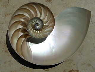
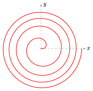
In mathematics, a spiral is a curve which emanates from a point, moving farther away as it revolves around the point. It is a subtype of whorled patterns, a broad group that also includes concentric objects.

A hyperbolic spiral is a plane curve, which can be described in polar coordinates by the equation
A Fermat's spiral or parabolic spiral is a plane curve with the property that the area between any two consecutive full turns around the spiral is invariant. As a result, the distance between turns grows in inverse proportion to their distance from the spiral center, contrasting with the Archimedean spiral and the logarithmic spiral. Fermat spirals are named after Pierre de Fermat.

In mathematics, a parametric equation defines a group of quantities as functions of one or more independent variables called parameters. Parametric equations are commonly used to express the coordinates of the points that make up a geometric object such as a curve or surface, called a parametric curve and parametric surface, respectively. In such cases, the equations are collectively called a parametric representation, or parametric system, or parameterization of the object.
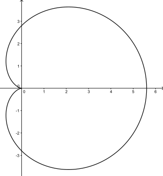
In geometry, a cardioid is a plane curve traced by a point on the perimeter of a circle that is rolling around a fixed circle of the same radius. It can also be defined as an epicycloid having a single cusp. It is also a type of sinusoidal spiral, and an inverse curve of the parabola with the focus as the center of inversion. A cardioid can also be defined as the set of points of reflections of a fixed point on a circle through all tangents to the circle.
In mathematics, specifically the study of differential equations, the Picard–Lindelöf theorem gives a set of conditions under which an initial value problem has a unique solution. It is also known as Picard's existence theorem, the Cauchy–Lipschitz theorem, or the existence and uniqueness theorem.

In geometry, a nephroid is a specific plane curve. It is a type of epicycloid in which the smaller circle's radius differs from the larger one by a factor of one-half.

In geometry, an envelope of a planar family of curves is a curve that is tangent to each member of the family at some point, and these points of tangency together form the whole envelope. Classically, a point on the envelope can be thought of as the intersection of two "infinitesimally adjacent" curves, meaning the limit of intersections of nearby curves. This idea can be generalized to an envelope of surfaces in space, and so on to higher dimensions.

The scale of a map is the ratio of a distance on the map to the corresponding distance on the ground. This simple concept is complicated by the curvature of the Earth's surface, which forces scale to vary across a map. Because of this variation, the concept of scale becomes meaningful in two distinct ways.
In calculus, the Leibniz integral rule for differentiation under the integral sign states that for an integral of the form
The gradient theorem, also known as the fundamental theorem of calculus for line integrals, says that a line integral through a gradient field can be evaluated by evaluating the original scalar field at the endpoints of the curve. The theorem is a generalization of the second fundamental theorem of calculus to any curve in a plane or space rather than just the real line.
There are several equivalent ways for defining trigonometric functions, and the proof of the trigonometric identities between them depend on the chosen definition. The oldest and somehow the most elementary definition is based on the geometry of right triangles. The proofs given in this article use this definition, and thus apply to non-negative angles not greater than a right angle. For greater and negative angles, see Trigonometric functions.
In mathematics, the differential geometry of surfaces deals with the differential geometry of smooth surfaces with various additional structures, most often, a Riemannian metric. Surfaces have been extensively studied from various perspectives: extrinsically, relating to their embedding in Euclidean space and intrinsically, reflecting their properties determined solely by the distance within the surface as measured along curves on the surface. One of the fundamental concepts investigated is the Gaussian curvature, first studied in depth by Carl Friedrich Gauss, who showed that curvature was an intrinsic property of a surface, independent of its isometric embedding in Euclidean space.
In geometry, a sectrix of Maclaurin is defined as the curve swept out by the point of intersection of two lines which are each revolving at constant rates about different points called poles. Equivalently, a sectrix of Maclaurin can be defined as a curve whose equation in biangular coordinates is linear. The name is derived from the trisectrix of Maclaurin, which is a prominent member of the family, and their sectrix property, which means they can be used to divide an angle into a given number of equal parts. There are special cases known as arachnida or araneidans because of their spider-like shape, and Plateau curves after Joseph Plateau who studied them.
In Euclidean geometry, for a plane curve C and a given fixed point O, the pedal equation of the curve is a relation between r and p where r is the distance from O to a point on C and p is the perpendicular distance from O to the tangent line to C at the point. The point O is called the pedal point and the values r and p are sometimes called the pedal coordinates of a point relative to the curve and the pedal point. It is also useful to measure the distance of O to the normal pc (the contrapedal coordinate) even though it is not an independent quantity and it relates to (r, p) as

In the geometry of curves, an orthoptic is the set of points for which two tangents of a given curve meet at a right angle.

The study of geodesics on an ellipsoid arose in connection with geodesy specifically with the solution of triangulation networks. The figure of the Earth is well approximated by an oblate ellipsoid, a slightly flattened sphere. A geodesic is the shortest path between two points on a curved surface, analogous to a straight line on a plane surface. The solution of a triangulation network on an ellipsoid is therefore a set of exercises in spheroidal trigonometry.

In differential geometry a translation surface is a surface that is generated by translations:
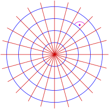


![Isogonal trajectories of concentric circles for
a
=
45
[?]
{\displaystyle \alpha =45^{\circ }} Kreise-isot.svg](http://upload.wikimedia.org/wikipedia/commons/thumb/b/be/Kreise-isot.svg/250px-Kreise-isot.svg.png)


