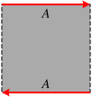
In mathematics, a projective plane is a geometric structure that extends the concept of a plane. In the ordinary Euclidean plane, two lines typically intersect at a single point, but there are some pairs of lines that do not intersect. A projective plane can be thought of as an ordinary plane equipped with additional "points at infinity" where parallel lines intersect. Thus any two distinct lines in a projective plane intersect at exactly one point.

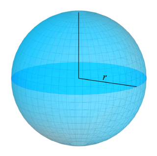
A sphere is a geometrical object that is a three-dimensional analogue to a two-dimensional circle. Formally, a sphere is the set of points that are all at the same distance r from a given point in three-dimensional space. That given point is the center of the sphere, and r is the sphere's radius. The earliest known mentions of spheres appear in the work of the ancient Greek mathematicians.

In mathematics, a 3-sphere, glome or hypersphere is a higher-dimensional analogue of a sphere. In 4-dimensional Euclidean space, it is the set of points equidistant from a fixed central point. Analogous to how the boundary of a ball in three dimensions is an ordinary sphere, the boundary of a ball in four dimensions is a 3-sphere. Topologically, a 3-sphere is an example of a 3-manifold, and it is also an n-sphere.
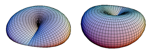
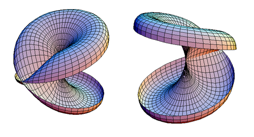
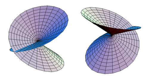
In mathematics, the Roman surface or Steiner surface is a self-intersecting mapping of the real projective plane into three-dimensional space, with an unusually high degree of symmetry. This mapping is not an immersion of the projective plane; however, the figure resulting from removing six singular points is one. Its name arises because it was discovered by Jakob Steiner when he was in Rome in 1844.
Elliptic geometry is an example of a geometry in which Euclid's parallel postulate does not hold. Instead, as in spherical geometry, there are no parallel lines since any two lines must intersect. However, unlike in spherical geometry, two lines are usually assumed to intersect at a single point. Because of this, the elliptic geometry described in this article is sometimes referred to as single elliptic geometry whereas spherical geometry is sometimes referred to as double elliptic geometry.

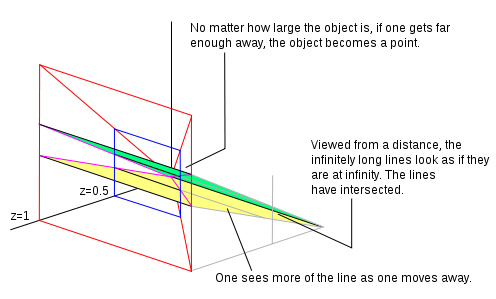
In mathematics, the concept of a projective space originated from the visual effect of perspective, where parallel lines seem to meet at infinity. A projective space may thus be viewed as the extension of a Euclidean space, or, more generally, an affine space with points at infinity, in such a way that there is one point at infinity of each direction of parallel lines.
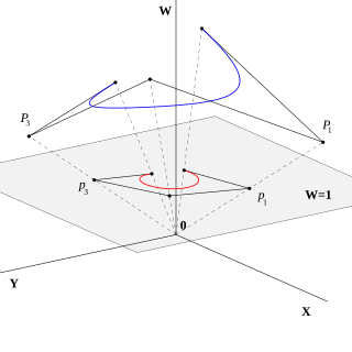
In mathematics, homogeneous coordinates or projective coordinates, introduced by August Ferdinand Möbius in his 1827 work Der barycentrische Calcul, are a system of coordinates used in projective geometry, just as Cartesian coordinates are used in Euclidean geometry. They have the advantage that the coordinates of points, including points at infinity, can be represented using finite coordinates. Formulas involving homogeneous coordinates are often simpler and more symmetric than their Cartesian counterparts. Homogeneous coordinates have a range of applications, including computer graphics and 3D computer vision, where they allow affine transformations and, in general, projective transformations to be easily represented by a matrix. They are also used in fundamental elliptic curve cryptography algorithms.
In geometry, an incidence relation is a heterogeneous relation that captures the idea being expressed when phrases such as "a point lies on a line" or "a line is contained in a plane" are used. The most basic incidence relation is that between a point, P, and a line, l, sometimes denoted P I l. If P I l the pair (P, l) is called a flag. There are many expressions used in common language to describe incidence (for example, a line passes through a point, a point lies in a plane, etc.) but the term "incidence" is preferred because it does not have the additional connotations that these other terms have, and it can be used in a symmetric manner. Statements such as "line l1 intersects line l2" are also statements about incidence relations, but in this case, it is because this is a shorthand way of saying that "there exists a point P that is incident with both line l1 and line l2". When one type of object can be thought of as a set of the other type of object (viz., a plane is a set of points) then an incidence relation may be viewed as containment.
In geometry and topology, the line at infinity is a projective line that is added to the real (affine) plane in order to give closure to, and remove the exceptional cases from, the incidence properties of the resulting projective plane. The line at infinity is also called the ideal line.
In projective geometry, a plane at infinity is the hyperplane at infinity of a three dimensional projective space or to any plane contained in the hyperplane at infinity of any projective space of higher dimension. This article will be concerned solely with the three-dimensional case.
In projective geometry, duality or plane duality is a formalization of the striking symmetry of the roles played by points and lines in the definitions and theorems of projective planes. There are two approaches to the subject of duality, one through language and the other a more functional approach through special mappings. These are completely equivalent and either treatment has as its starting point the axiomatic version of the geometries under consideration. In the functional approach there is a map between related geometries that is called a duality. Such a map can be constructed in many ways. The concept of plane duality readily extends to space duality and beyond that to duality in any finite-dimensional projective geometry.
In linear algebra, linear transformations can be represented by matrices. If is a linear transformation mapping to and is a column vector with entries, then for some matrix , called the transformation matrix of . Note that has rows and columns, whereas the transformation is from to . There are alternative expressions of transformation matrices involving row vectors that are preferred by some authors.
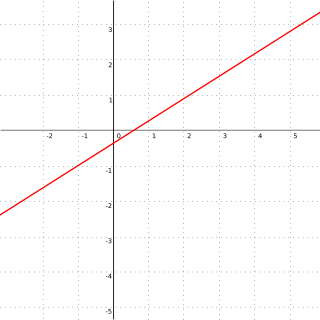
In geometry, a straight line, usually abbreviated line, is an infinitely long object with no width, depth, or curvature, an idealization of such physical objects as a straightedge, a taut string, or a ray of light. Lines are spaces of dimension one, which may be embedded in spaces of dimension two, three, or higher. The word line may also refer, in everyday life, to a line segment, which is a part of a line delimited by two points.
In multilinear algebra, a multivector, sometimes called Clifford number or multor, is an element of the exterior algebra Λ(V) of a vector space V. This algebra is graded, associative and alternating, and consists of linear combinations of simplek-vectors (also known as decomposablek-vectors or k-blades) of the form

In geometry, a pencil is a family of geometric objects with a common property, for example the set of lines that pass through a given point in a plane, or the set of circles that pass through two given points in a plane.

The Lambert azimuthal equal-area projection is a particular mapping from a sphere to a disk. It accurately represents area in all regions of the sphere, but it does not accurately represent angles. It is named for the Swiss mathematician Johann Heinrich Lambert, who announced it in 1772. "Zenithal" being synonymous with "azimuthal", the projection is also known as the Lambert zenithal equal-area projection.
In mathematics, a surface is a mathematical model of the common concept of a surface. It is a generalization of a plane, but, unlike a plane, it may be curved; this is analogous to a curve generalizing a straight line.
In projective geometry, the circular points at infinity are two special points at infinity in the complex projective plane that are contained in the complexification of every real circle.
In mathematics, the differential geometry of surfaces deals with the differential geometry of smooth surfaces with various additional structures, most often, a Riemannian metric.
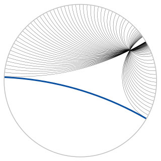
In geometry, the Poincaré disk model, also called the conformal disk model, is a model of 2-dimensional hyperbolic geometry in which all points are inside the unit disk, and straight lines are either circular arcs contained within the disk that are orthogonal to the unit circle or diameters of the unit circle.