Jordan curve theorem

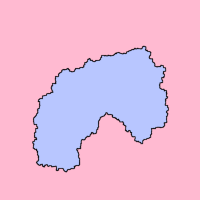
Illustration of the Jordan curve theorem. The Jordan curve (drawn in black) divides the plane into an "inside" region (light blue) and an "outside" region (pink).

In topology, the Jordan curve theorem asserts that every Jordan curve (a plane simple closed curve) divides the plane into an "interior" region bounded by the curve and an "exterior" region containing all of the nearby and far away exterior points. Every continuous path connecting a point of one region to a point of the other intersects with the curve somewhere. While the theorem seems intuitively obvious, it takes some ingenuity to prove it by elementary means. "Although the JCT is one of the best known topological theorems, there are many, even among professional mathematicians, who have never read a proof of it." (Tverberg (1980 , Introduction)). More transparent proofs rely on the mathematical machinery of algebraic topology, and these lead to generalizations to higher-dimensional spaces.

The Jordan curve theorem is named after the mathematician Camille Jordan (1838–1922), who published its first claimed proof in 1887. ^{[1] [2]} For decades, mathematicians generally thought that this proof was flawed and that the first rigorous proof was carried out by Oswald Veblen. However, this notion has been overturned by Thomas C. Hales and others. ^[3]

Definitions and the statement of the Jordan theorem

A Jordan curve or a simple closed curve in the plane R² is the image C of an injective continuous map of a circle into the plane, φ: S¹ → R². A Jordan arc in the plane is the image of an injective continuous map of a closed and bounded interval [a, b] into the plane. It is a plane curve that is not necessarily smooth nor algebraic.

Alternatively, a Jordan curve is the image of a continuous map φ: [0,1] → R² such that φ(0) = φ(1) and the restriction of φ to [0,1) is injective. The first two conditions say that C is a continuous loop, whereas the last condition stipulates that C has no self-intersection points.

With these definitions, the Jordan curve theorem can be stated as follows:

Theorem — Let C be a Jordan curve in the plane R². Then its complement, R² \ C, consists of exactly two connected components. One of these components is bounded (the interior) and the other is unbounded (the exterior), and the curve C is the boundary of each component.

In contrast, the complement of a Jordan arc in the plane is connected.

Proof and generalizations

The Jordan curve theorem was independently generalized to higher dimensions by H. Lebesgue and L. E. J. Brouwer in 1911, resulting in the Jordan–Brouwer separation theorem.

Theorem — Let X be an n-dimensional topological sphere in the (n+1)-dimensional Euclidean space Rⁿ⁺¹ (n > 0), i.e. the image of an injective continuous mapping of the n-sphere Sⁿ into Rⁿ⁺¹. Then the complement Y of X in Rⁿ⁺¹ consists of exactly two connected components. One of these components is bounded (the interior) and the other is unbounded (the exterior). The set X is their common boundary.

The proof uses homology theory. It is first established that, more generally, if X is homeomorphic to the k-sphere, then the reduced integral homology groups of Y = Rⁿ⁺¹ \ X are as follows:

$${\displaystyle {\tilde {H}}_{q}(Y)={\begin{cases}\mathbb {Z} ,&q=n-k{\text{ or }}q=n,\\\{0\},&{\text{otherwise}}.\end{cases}}}$$

This is proved by induction in k using the Mayer–Vietoris sequence. When n = k, the zeroth reduced homology of Y has rank 1, which means that Y has 2 connected components (which are, moreover, path connected), and with a bit of extra work, one shows that their common boundary is X. A further generalization was found by J. W. Alexander, who established the Alexander duality between the reduced homology of a compact subset X of Rⁿ⁺¹ and the reduced cohomology of its complement. If X is an n-dimensional compact connected submanifold of Rⁿ⁺¹ (or Sⁿ⁺¹) without boundary, its complement has 2 connected components.

There is a strengthening of the Jordan curve theorem, called the Jordan–Schönflies theorem, which states that the interior and the exterior planar regions determined by a Jordan curve in R² are homeomorphic to the interior and exterior of the unit disk. In particular, for any point P in the interior region and a point A on the Jordan curve, there exists a Jordan arc connecting P with A and, with the exception of the endpoint A, completely lying in the interior region. An alternative and equivalent formulation of the Jordan–Schönflies theorem asserts that any Jordan curve φ: S¹ → R², where S¹ is viewed as the unit circle in the plane, can be extended to a homeomorphism ψ: R² → R² of the plane. Unlike Lebesgue's and Brouwer's generalization of the Jordan curve theorem, this statement becomes false in higher dimensions: while the exterior of the unit ball in R³ is simply connected, because it retracts onto the unit sphere, the Alexander horned sphere is a subset of R³ homeomorphic to a sphere, but so twisted in space that the unbounded component of its complement in R³ is not simply connected, and hence not homeomorphic to the exterior of the unit ball.

Discrete version

The Jordan curve theorem can be proved from the Brouwer fixed point theorem (in 2 dimensions), ^[4] and the Brouwer fixed point theorem can be proved from the Hex theorem: "every game of Hex has at least one winner", from which we obtain a logical implication: Hex theorem implies Brouwer fixed point theorem, which implies Jordan curve theorem. ^[5]

It is clear that Jordan curve theorem implies the "strong Hex theorem": "every game of Hex ends with exactly one winner, with no possibility of both sides losing or both sides winning", thus the Jordan curve theorem is equivalent to the strong Hex theorem, which is a purely discrete theorem.

The Brouwer fixed point theorem, by being sandwiched between the two equivalent theorems, is also equivalent to both. ^[6]

In reverse mathematics, and computer-formalized mathematics, the Jordan curve theorem is commonly proved by first converting it to an equivalent discrete version similar to the strong Hex theorem, then proving the discrete version. ^[7]

Application to image processing

In image processing, a binary picture is a discrete square grid of 0 and 1, or equivalently, a compact subset of ${\displaystyle \mathbb {Z} ^{2}}$. Topological invariants on ${\displaystyle \mathbb {R} ^{2}}$, such as number of components, might fail to be well-defined for ${\displaystyle \mathbb {Z} ^{2}}$ if ${\displaystyle \mathbb {Z} ^{2}}$ does not have an appropriately defined graph structure.

There are two obvious graph structures on ${\displaystyle \mathbb {Z} ^{2}}$:

8-neighbor and 4-neighbor square grids.

• the "4-neighbor square grid", where each vertex ${\displaystyle (x,y)}$ is connected with ${\displaystyle (x+1,y),(x-1,y),(x,y+1),(x,y-1)}$.
• the "8-neighbor square grid", where each vertex ${\displaystyle (x,y)}$ is connected with ${\displaystyle (x',y')}$ iff ${\displaystyle |x-x'|\leq 1,|y-y'|\leq 1}$, and ${\displaystyle (x,y)\neq (x',y')}$.

Both graph structures fail to satisfy the strong Hex theorem. The 4-neighbor square grid allows a no-winner situation, and the 8-neighbor square grid allows a two-winner situation. Consequently, connectedness properties in ${\displaystyle \mathbb {R} ^{2}}$, such as the Jordan curve theorem, do not generalize to ${\displaystyle \mathbb {Z} ^{2}}$ under either graph structure.

If the "6-neighbor square grid" structure is imposed on ${\displaystyle \mathbb {Z} ^{2}}$, then it is the hexagonal grid, and thus satisfies the strong Hex theorem, allowing the Jordan curve theorem to generalize. For this reason, when computing connected components in a binary image, the 6-neighbor square grid is generally used. ^[8]

Steinhaus chessboard theorem

The Steinhaus chessboard theorem in some sense shows that the 4-neighbor grid and the 8-neighbor grid "together" implies the Jordan curve theorem, and the 6-neighbor grid is a precise interpolation between them. ^{[9] [10]}

The theorem states that: suppose you put bombs on some squares on a ${\displaystyle n\times n}$ chessboard, so that a king cannot move from the bottom side to the top side without stepping on a bomb, then a rook can move from the left side to the right side stepping only on bombs.

History and further proofs

The statement of the Jordan curve theorem may seem obvious at first, but it is a rather difficult theorem to prove. Bernard Bolzano was the first to formulate a precise conjecture, observing that it was not a self-evident statement, but that it required a proof. ^[11] It is easy to establish this result for polygons, but the problem came in generalizing it to all kinds of badly behaved curves, which include nowhere differentiable curves, such as the Koch snowflake and other fractal curves, or even a Jordan curve of positive area constructed by Osgood (1903).

The first proof of this theorem was given by Camille Jordan in his lectures on real analysis, and was published in his book Cours d'analyse de l'École Polytechnique. ^[1] There is some controversy about whether Jordan's proof was complete: the majority of commenters on it have claimed that the first complete proof was given later by Oswald Veblen, who said the following about Jordan's proof:

His proof, however, is unsatisfactory to many mathematicians. It assumes the theorem without proof in the important special case of a simple polygon, and of the argument from that point on, one must admit at least that all details are not given. ^[12]

However, Thomas C. Hales wrote:

Nearly every modern citation that I have found agrees that the first correct proof is due to Veblen... In view of the heavy criticism of Jordan’s proof, I was surprised when I sat down to read his proof to find nothing objectionable about it. Since then, I have contacted a number of the authors who have criticized Jordan, and each case the author has admitted to having no direct knowledge of an error in Jordan’s proof. ^[13]

Hales also pointed out that the special case of simple polygons is not only an easy exercise, but was not really used by Jordan anyway, and quoted Michael Reeken as saying:

Jordan’s proof is essentially correct... Jordan’s proof does not present the details in a satisfactory way. But the idea is right, and with some polishing the proof would be impeccable. ^[14]

Earlier, Jordan's proof and another early proof by Charles Jean de la Vallée Poussin had already been critically analyzed and completed by Schoenflies (1924). ^[15]

Due to the importance of the Jordan curve theorem in low-dimensional topology and complex analysis, it received much attention from prominent mathematicians of the first half of the 20th century. Various proofs of the theorem and its generalizations were constructed by J. W. Alexander, Louis Antoine, Ludwig Bieberbach, Luitzen Brouwer, Arnaud Denjoy, Friedrich Hartogs, Béla Kerékjártó, Alfred Pringsheim, and Arthur Moritz Schoenflies.

New elementary proofs of the Jordan curve theorem, as well as simplifications of the earlier proofs, continue to be carried out.

• Elementary proofs were presented by Filippov (1950) and Tverberg (1980).
• A proof using non-standard analysis by Narens (1971).
• A proof using constructive mathematics by Gordon O.Berg,W. Julian,andR. Mineset al. ( 1975 ).
• A proof using the Brouwer fixed point theorem by Maehara (1984).
• A proof using non-planarity of the complete bipartite graph K_3,3 was given by Thomassen (1992).

The root of the difficulty is explained in Tverberg (1980) as follows. It is relatively simple to prove that the Jordan curve theorem holds for every Jordan polygon (Lemma 1), and every Jordan curve can be approximated arbitrarily well by a Jordan polygon (Lemma 2). A Jordan polygon is a polygonal chain, the boundary of a bounded connected open set, call it the open polygon, and its closure, the closed polygon. Consider the diameter ${\displaystyle \delta }$ of the largest disk contained in the closed polygon. Evidently, ${\displaystyle \delta }$ is positive. Using a sequence of Jordan polygons (that converge to the given Jordan curve) we have a sequence ${\displaystyle \delta _{1},\delta _{2},\dots }$presumably converging to a positive number, the diameter ${\displaystyle \delta }$ of the largest disk contained in the closed region bounded by the Jordan curve. However, we have to prove that the sequence ${\displaystyle \delta _{1},\delta _{2},\dots }$ does not converge to zero, using only the given Jordan curve, not the region presumably bounded by the curve. This is the point of Tverberg's Lemma 3. Roughly, the closed polygons should not thin to zero everywhere. Moreover, they should not thin to zero somewhere, which is the point of Tverberg's Lemma 4.

The first formal proof of the Jordan curve theorem was created by Hales (2007a) in the HOL Light system, in January 2005, and contained about 60,000 lines. Another rigorous 6,500-line formal proof was produced in 2005 by an international team of mathematicians using the Mizar system. Both the Mizar and the HOL Light proof rely on libraries of previously proved theorems, so these two sizes are not comparable. NobuyukiSakamotoandKeita Yokoyama ( 2007 ) showed that in reverse mathematics the Jordan curve theorem is equivalent to weak Kőnig's lemma over the system ${\displaystyle {\mathsf {RCA}}_{0}}$.

Application

If the initial point (p_a) of a ray (in red) lies outside a simple polygon (region A), the number of intersections of the ray and the polygon is even.
If the initial point (p_b) of a ray lies inside the polygon (region B), the number of intersections is odd.

Main article: Point in polygon § Ray casting algorithm

In computational geometry, the Jordan curve theorem can be used for testing whether a point lies inside or outside a simple polygon. ^{[16] [17] [18]}

From a given point, trace a ray that does not pass through any vertex of the polygon (all rays but a finite number are convenient). Then, compute the number n of intersections of the ray with an edge of the polygon. Jordan curve theorem proof implies that the point is inside the polygon if and only if n is odd.

Computational aspects

Adler, Daskalakis and Demaine ^[19] prove that a computational version of Jordan’s theorem is PPAD-complete. As a corollary, they show that Jordan's theorem implies the Brouwer fixed-point theorem. This complements the earlier result by Maehara, that Brouwer's fixed point theorem implies Jordan's theorem. ^[20]

See also

• Denjoy–Riesz theorem, a description of certain sets of points in the plane that can be subsets of Jordan curves
• Lakes of Wada
• Quasi-Fuchsian group, a mathematical group that preserves a Jordan curve

Notes

1. Jordan (1887).
2. Kline, J. R. (1942). "What is the Jordan curve theorem?". American Mathematical Monthly. 49: 281–286. doi:10.2307/2303093. MR   0006516.
3. Hales, Thomas C. (2007). "Jordan's proof of the Jordan curve theorem" (PDF). From Insight to Proof: Festschrift in Honour of Andrzej Trybulec. Studies in Logic, Grammar and Rhetoric. University of Białystok. 10 (23).
4. Maehara (1984), p. 641.
5. Gale, David (December 1979). "The Game of Hex and the Brouwer Fixed-Point Theorem". The American Mathematical Monthly. 86 (10): 818–827. doi:10.2307/2320146. ISSN   0002-9890. JSTOR   2320146.
6. Nguyen, Phuong; Cook, Stephen A. (2007). "The Complexity of Proving the Discrete Jordan Curve Theorem". 22nd Annual IEEE Symposium on Logic in Computer Science (LICS 2007). IEEE. pp. 245–256. arXiv: 1002.2954 . doi:10.1109/lics.2007.48. ISBN   978-0-7695-2908-0.
7. Hales, Thomas C. (December 2007). "The Jordan Curve Theorem, Formally and Informally". The American Mathematical Monthly. 114 (10): 882–894. doi:10.1080/00029890.2007.11920481. ISSN   0002-9890. S2CID   887392.
8. Nayar, Shree (Mar 1, 2021). "First Principles of Computer Vision: Segmenting Binary Images | Binary Images". YouTube .
9. Šlapal, J (April 2004). "A digital analogue of the Jordan curve theorem". Discrete Applied Mathematics. 139 (1–3): 231–251. doi: 10.1016/j.dam.2002.11.003 . ISSN   0166-218X.
10. Surówka, Wojciech (1993). "A discrete form of Jordan curve theorem". Annales Mathematicae Silesianae (7): 57–61. MR   1271184.
11. Johnson, Dale M. (1977). "Prelude to dimension theory: the geometrical investigations of Bernard Bolzano". Archive for History of Exact Sciences. 17 (3): 262–295. doi:10.1007/BF00499625. MR   0446838. See p. 285.
12. OswaldVeblen  ( 1905 )
13. Hales (2007b)
14. Hales (2007b)
15. A. Schoenflies (1924). "Bemerkungen zu den Beweisen von C. Jordan und Ch. J. de la Vallée Poussin". Jahresber. Deutsch. Math.-Verein. 33: 157–160.
16. RichardCourant ( 1978 )
17. "V. Topology". 1. Jordan curve theorem (PDF). Edinburg: University of Edinburgh. 1978. p. 267.
18. "PNPOLY - Point Inclusion in Polygon Test - WR Franklin (WRF)". wrf.ecse.rpi.edu. Retrieved 2021-07-18.
19. Adler, Aviv; Daskalakis, Constantinos; Demaine, Erik D. (2016). Chatzigiannakis, Ioannis; Mitzenmacher, Michael; Rabani, Yuval; Sangiorgi, Davide (eds.). "The Complexity of Hex and the Jordan Curve Theorem". 43rd International Colloquium on Automata, Languages, and Programming (ICALP 2016). Leibniz International Proceedings in Informatics (LIPIcs). Dagstuhl, Germany: Schloss Dagstuhl–Leibniz-Zentrum fuer Informatik. 55: 24:1–24:14. doi:10.4230/LIPIcs.ICALP.2016.24. ISBN   978-3-95977-013-2.
20. Maehara (1984).

References

• Berg, Gordon O.; Julian, W.; Mines, R.; Richman, Fred (1975), "The constructive Jordan curve theorem", Rocky Mountain Journal of Mathematics , 5 (2): 225–236, doi: 10.1216/RMJ-1975-5-2-225 , ISSN   0035-7596, MR   0410701
• Courant, Richard (1978). "V. Topology". Written at Oxford. What is mathematics? : an elementary approach to ideas and methods . Herbert Robbins ([4th ed.] ed.). United Kingdom: Oxford University Press. p. 267. ISBN   978-0-19-502517-0. OCLC   6450129.
• Filippov, A. F. (1950), "An elementary proof of Jordan's theorem" (PDF), Uspekhi Mat. Nauk (in Russian), 5 (5): 173–176
• Hales, Thomas C. (2007a), "The Jordan curve theorem, formally and informally", The American Mathematical Monthly , 114 (10): 882–894, doi:10.1080/00029890.2007.11920481, ISSN   0002-9890, MR   2363054, S2CID   887392
• Hales, Thomas (2007b), "Jordan's proof of the Jordan Curve theorem" (PDF), Studies in Logic, Grammar and Rhetoric, 10 (23)
• Jordan, Camille (1887), Cours d'analyse (PDF), pp. 587–594
• Maehara, Ryuji (1984), "The Jordan Curve Theorem Via the Brouwer Fixed Point Theorem", The American Mathematical Monthly , 91 (10): 641–643, doi:10.2307/2323369, ISSN   0002-9890, JSTOR   2323369, MR   0769530
• Narens, Louis (1971), "A nonstandard proof of the Jordan curve theorem", Pacific Journal of Mathematics , 36: 219–229, doi: 10.2140/pjm.1971.36.219 , ISSN   0030-8730, MR   0276940
• Osgood, William F. (1903), "A Jordan Curve of Positive Area", Transactions of the American Mathematical Society , 4 (1): 107–112, doi: 10.2307/1986455 , ISSN   0002-9947, JFM   34.0533.02, JSTOR   1986455
• Ross, Fiona; Ross, William T. (2011), "The Jordan curve theorem is non-trivial", Journal of Mathematics and the Arts , 5 (4): 213–219, doi:10.1080/17513472.2011.634320, S2CID   3257011 . author's site
• Sakamoto, Nobuyuki; Yokoyama, Keita (2007), "The Jordan curve theorem and the Schönflies theorem in weak second-order arithmetic", Archive for Mathematical Logic, 46 (5): 465–480, doi:10.1007/s00153-007-0050-6, ISSN   0933-5846, MR   2321588, S2CID   33627222
• Thomassen, Carsten (1992), "The Jordan–Schönflies theorem and the classification of surfaces", American Mathematical Monthly, 99 (2): 116–130, doi:10.2307/2324180, JSTOR   2324180
• Tverberg, Helge (1980), "A proof of the Jordan curve theorem" (PDF), Bulletin of the London Mathematical Society , 12 (1): 34–38, CiteSeerX   10.1.1.374.2903 , doi:10.1112/blms/12.1.34
• Veblen, Oswald (1905), "Theory on Plane Curves in Non-Metrical Analysis Situs", Transactions of the American Mathematical Society , 6 (1): 83–98, doi: 10.2307/1986378 , JSTOR   1986378, MR   1500697

External links

• M.I. Voitsekhovskii (2001) [1994], "Jordan theorem", Encyclopedia of Mathematics , EMS Press
• The full 6,500 line formal proof of Jordan's curve theorem in Mizar.
• Collection of proofs of the Jordan curve theorem at Andrew Ranicki's homepage
• A simple proof of Jordan curve theorem (PDF) by David B. Gauld
• Brown, R.; Antolino-Camarena, O. (2014). "Corrigendum to "Groupoids, the Phragmen-Brouwer Property, and the Jordan Curve Theorem", J. Homotopy and Related Structures 1 (2006) 175-183". arXiv: 1404.0556 [math.AT].