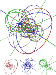
2-sphere wireframe as an orthogonal projectionJust as a stereographic projection can project a sphere's surface to a plane, it can also project a 3-sphere into 3-space. This image shows three coordinate directions projected to 3-space: parallels (red), meridians (blue), and hypermeridians (green). Due to the conformal property of the stereographic projection, the curves intersect each other orthogonally (in the yellow points) as in 4D. All of the curves are circles: the curves that intersect ⟨0,0,0,1⟩ have an infinite radius (= straight line).
Considered extrinsically, as a hypersurface embedded in (n+1)-dimensional Euclidean space, an n-sphere is the locus of points at equal distance (the radius) from a given center point. Its interior, consisting of all points closer to the center than the radius, is an (n+1)-dimensional ball. In particular:
The 0-sphere is the pair of points at the ends of a line segment (1-ball).
In the more general setting of topology, any topological space that is homeomorphic to the unit n-sphere is called an n-sphere. Under inverse stereographic projection, the n-sphere is the one-point compactification of n-space. The n-spheres admit several other topological descriptions: for example, they can be constructed by gluing two n-dimensional spaces together, by identifying the boundary of an n-cube with a point, or (inductively) by forming the suspension of an (n−1)-sphere. When n ≥ 2 it is simply connected; the 1-sphere (circle) is not simply connected; the 0-sphere is not even connected, consisting of two discrete points.
Description
For any natural numbern, an n-sphere of radius r is defined as the set of points in (n + 1)-dimensional Euclidean space that are at distance r from some fixed point c, where r may be any positivereal number and where c may be any point in (n + 1)-dimensional space. In particular:
a 0-sphere is a pair of points {c − r, c + r}, and is the boundary of a line segment (1-ball).
a 1-sphere is a circle of radius r centered at c, and is the boundary of a disk (2-ball).
a 2-sphere is an ordinary 2-dimensional sphere in 3-dimensional Euclidean space, and is the boundary of an ordinary ball (3-ball).
a 3-sphere is a 3-dimensional sphere in 4-dimensional Euclidean space.
Cartesian coordinates
The set of points in (n + 1)-space, (x1, x2, ..., xn+1), that define an n-sphere, Sn(r), is represented by the equation:
where c = (c1, c2, ..., cn+1) is a center point, and r is the radius.
The above n-sphere exists in (n + 1)-dimensional Euclidean space and is an example of an n-manifold. The volume formω of an n-sphere of radius r is given by
where is the Hodge star operator; see Flanders (1989, §6.1) for a discussion and proof of this formula in the case r = 1. As a result,
The space enclosed by an n-sphere is called an (n + 1)-ball. An (n + 1)-ball is closed if it includes the n-sphere, and it is open if it does not include the n-sphere.
Specifically:
A 1-ball, a line segment, is the interior of a 0-sphere.
A 2-ball, a disk, is the interior of a circle (1-sphere).
A 3-ball, an ordinary ball, is the interior of a sphere (2-sphere).
Topologically, an n-sphere can be constructed as a one-point compactification of n-dimensional Euclidean space. Briefly, the n-sphere can be described as Sn = ℝn ∪ {∞}, which is n-dimensional Euclidean space plus a single point representing infinity in all directions. In particular, if a single point is removed from an n-sphere, it becomes homeomorphic to ℝn. This forms the basis for stereographic projection.[1]
Let Sn−1 be the surface area of the unit (n−1)-sphere of radius 1 embedded in n-dimensional Euclidean space, and let Vn be the volume of its interior, the unit n-ball. The surface area of an arbitrary (n−1)-sphere is proportional to the (n−1)st power of the radius, and the volume of an arbitrary n-ball is proportional to the nth power of the radius.
The 0-ball is sometimes defined as a single point. The 0-dimensional Hausdorff measure is the number of points in a set. So
A unit 1-ball is a line segment whose points have a single coordinate in the interval [−1, 1] of length 2, and the 0-sphere consists of its two end-points, with coordinate {−1, 1}.
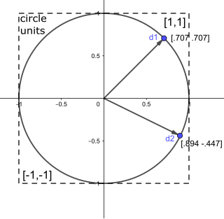
A unit 1-sphere is the unit circle in the Euclidean plane, and its interior is the unit disk (2-ball).
As n tends to infinity, the volume of the unit n-ball (ratio between the volume of an n-ball of radius 1 and an n-cube of side length 1) tends to zero.[2]
Recurrences
The surface area, or properly the n-dimensional volume, of the n-sphere at the boundary of the (n + 1)-ball of radius R is related to the volume of the ball by the differential equation
Equivalently, representing the unit n-ball as a union of concentric (n − 1)-sphere shells,
We can also represent the unit (n + 2)-sphere as a union of products of a circle (1-sphere) with an n-sphere. Then Since S1 = 2π V0, the equation
holds for all n. Along with the base cases from above, these recurrences can be used to compute the surface area of any sphere or volume of any ball.
Spherical coordinates
We may define a coordinate system in an n-dimensional Euclidean space which is analogous to the spherical coordinate system defined for 3-dimensional Euclidean space, in which the coordinates consist of a radial coordinate r, and n − 1 angular coordinates φ1, φ2, ..., φn−1, where the angles φ1, φ2, ..., φn−2 range over [0, π] radians (or over [0, 180] degrees) and φn−1 ranges over [0, 2π) radians (or over [0, 360) degrees). If xi are the Cartesian coordinates, then we may compute x1, ..., xn from r, φ1, ..., φn−1 with:[3]
Except in the special cases described below, the inverse transformation is unique:
where atan2 is the two-argument arctangent function.
There are some special cases where the inverse transform is not unique; φk for any k will be ambiguous whenever all of xk, xk+1, ... xn are zero; in this case φk may be chosen to be zero. (For example, for the 2-sphere, when the polar angle is 0 or π then the point is one of the poles, zenith or nadir, and the choice of azimuthal angle is arbitrary.)
Spherical volume and area elements
To express the volume element of n-dimensional Euclidean space in terms of spherical coordinates, let and for concision, then observe that the Jacobian matrix of the transformation is:
The determinant of this matrix can be calculated by induction. When n = 2, a straightforward computation shows that the determinant is r. For larger n, observe that Jn can be constructed from Jn−1 as follows. Except in column n, rows n− 1 and n of Jn are the same as row n− 1 of Jn−1, but multiplied by an extra factor of cos φn−1 in row n− 1 and an extra factor of sin φn−1 in row n. In column n, rows n− 1 and n of Jn are the same as column n− 1 of row n− 1 of Jn−1, but multiplied by extra factors of sin φn−1 in row n− 1 and cos φn−1 in row n, respectively. The determinant of Jn can be calculated by Laplace expansion in the final column. By the recursive description of Jn, the submatrix formed by deleting the entry at (n− 1, n) and its row and column almost equals Jn−1, except that its last row is multiplied by sin φn−1. Similarly, the submatrix formed by deleting the entry at (n, n) and its row and column almost equals Jn−1, except that its last row is multiplied by cos φn−1. Therefore the determinant of Jn is
Induction then gives a closed-form expression for the volume element in spherical coordinates
The formula for the volume of the n-ball can be derived from this by integration.
Similarly the surface area element of the (n − 1)-sphere of radius R, which generalizes the area element of the 2-sphere, is given by
The natural choice of an orthogonal basis over the angular coordinates is a product of ultraspherical polynomials,
for j = 1, 2, ..., n − 2, and the eisφj for the angle j = n − 1 in concordance with the spherical harmonics.
Polyspherical coordinates
The standard spherical coordinate system arises from writing ℝn as the product ℝ × ℝn−1. These two factors may be related using polar coordinates. For each point x of ℝn, the standard Cartesian coordinates
can be transformed into a mixed polar–Cartesian coordinate system:
This says that points in ℝn may be expressed by taking the ray starting at the origin and passing through , rotating it towards by , and traveling a distance along the ray. Repeating this decomposition eventually leads to the standard spherical coordinate system.
Polyspherical coordinate systems arise from a generalization of this construction.[4] The space ℝn is split as the product of two Euclidean spaces of smaller dimension, but neither space is required to be a line. Specifically, suppose that p and q are positive integers such that n = p + q. Then ℝn = ℝp× ℝq. Using this decomposition, a point x ∈ ℝn may be written as
This can be transformed into a mixed polar–Cartesian coordinate system by writing:
Here and are the unit vectors associated to y and z. This expresses x in terms of , , r ≥ 0, and an angle θ. It can be shown that the domain of θ is [0, 2π) if p = q = 1, [0, π] if exactly one of p and q is 1, and [0, π/2] if neither p nor q are 1. The inverse transformation is
These splittings may be repeated as long as one of the factors involved has dimension two or greater. A polyspherical coordinate system is the result of repeating these splittings until there are no Cartesian coordinates left. Splittings after the first do not require a radial coordinate because the domains of and are spheres, so the coordinates of a polyspherical coordinate system are a non-negative radius and n− 1 angles. The possible polyspherical coordinate systems correspond to binary trees with n leaves. Each non-leaf node in the tree corresponds to a splitting and determines an angular coordinate. For instance, the root of the tree represents ℝn, and its immediate children represent the first splitting into ℝp and ℝq. Leaf nodes correspond to Cartesian coordinates for Sn−1. The formulas for converting from polyspherical coordinates to Cartesian coordinates may be determined by finding the paths from the root to the leaf nodes. These formulas are products with one factor for each branch taken by the path. For a node whose corresponding angular coordinate is θi, taking the left branch introduces a factor of sin θi and taking the right branch introduces a factor of cos θi. The inverse transformation, from polyspherical coordinates to Cartesian coordinates, is determined by grouping nodes. Every pair of nodes having a common parent can be converted from a mixed polar–Cartesian coordinate system to a Cartesian coordinate system using the above formulas for a splitting.
Polyspherical coordinates also have an interpretation in terms of the special orthogonal group. A splitting ℝn = ℝp× ℝq determines a subgroup
This is the subgroup that leaves each of the two factors fixed. Choosing a set of coset representatives for the quotient is the same as choosing representative angles for this step of the polyspherical coordinate decomposition.
In polyspherical coordinates, the volume measure on ℝn and the area measure on Sn−1 are products. There is one factor for each angle, and the volume measure on ℝn also has a factor for the radial coordinate. The area measure has the form:
where the factors Fi are determined by the tree. Similarly, the volume measure is
Suppose we have a node of the tree that corresponds to the decomposition ℝn1+n2 = ℝn1 × ℝn2 and that has angular coordinate θ. The corresponding factor F depends on the values of n1 and n2. When the area measure is normalized so that the area of the sphere is 1, these factors are as follows. If n1 = n2 = 1, then
If n1 > 1 and n2 = 1, and if B denotes the beta function, then
If n1 = 1 and n2 > 1, then
Finally, if both n1 and n2 are greater than one, then
Just as a two-dimensional sphere embedded in three dimensions can be mapped onto a two-dimensional plane by a stereographic projection, an n-sphere can be mapped onto an n-dimensional hyperplane by the n-dimensional version of the stereographic projection. For example, the point [x,y,z] on a two-dimensional sphere of radius 1 maps to the point [x/1 − z, y/1 − z] on the xy-plane. In other words,
Likewise, the stereographic projection of an n-sphere Sn of radius 1 will map to the (n − 1)-dimensional hyperplane ℝn−1 perpendicular to the xn-axis as
Probability distributions
Uniformly at random on the (n − 1)-sphere
A set of points drawn from a uniform distribution on the surface of a unit 2-sphere, generated using Marsaglia's algorithm.
To generate uniformly distributed random points on the unit (n − 1)-sphere (that is, the surface of the unit n-ball), Marsaglia (1972) gives the following algorithm.
Generate an n-dimensional vector of normal deviates (it suffices to use N(0, 1), although in fact the choice of the variance is arbitrary), x = (x1, x2, ..., xn). Now calculate the "radius" of this point:
The vector 1/rx is uniformly distributed over the surface of the unit n-ball.
An alternative given by Marsaglia is to uniformly randomly select a point x = (x1, x2, ..., xn) in the unit n-cube by sampling each xi independently from the uniform distribution over (–1, 1), computing r as above, and rejecting the point and resampling if r ≥ 1 (i.e., if the point is not in the n-ball), and when a point in the ball is obtained scaling it up to the spherical surface by the factor 1/r; then again 1/rx is uniformly distributed over the surface of the unit n-ball. This method becomes very inefficient for higher dimensions, as a vanishingly small fraction of the unit cube is contained in the sphere. In ten dimensions, less than 2% of the cube is filled by the sphere, so that typically more than 50 attempts will be needed. In seventy dimensions, less than of the cube is filled, meaning typically a trillion quadrillion trials will be needed, far more than a computer could ever carry out.
Uniformly at random within the n-ball
With a point selected uniformly at random from the surface of the unit (n − 1)-sphere (e.g., by using Marsaglia's algorithm), one needs only a radius to obtain a point uniformly at random from within the unit n-ball. If u is a number generated uniformly at random from the interval [0, 1] and x is a point selected uniformly at random from the unit (n − 1)-sphere, then u1/nx is uniformly distributed within the unit n-ball.
Alternatively, points may be sampled uniformly from within the unit n-ball by a reduction from the unit (n + 1)-sphere. In particular, if (x1, x2, ..., xn+2) is a point selected uniformly from the unit (n + 1)-sphere, then (x1, x2, ..., xn) is uniformly distributed within the unit n-ball (i.e., by simply discarding two coordinates).[5]
If n is sufficiently large, most of the volume of the n-ball will be contained in the region very close to its surface, so a point selected from that volume will also probably be close to the surface. This is one of the phenomena leading to the so-called curse of dimensionality that arises in some numerical and other applications.
Distribution of the first coordinate
Let be the square of the first coordinate of a point sampled uniformly at random from the (n-1)-sphere, then its probability density function, for , is
Let be the appropriately scaled version, then at the limit, the probability density function of converges to . This is sometimes called the Porter–Thomas distribution.[6]
PrincipalU(1)-bundle over CP2. SO(6) / SO(5) = SU(3) / SU(2). It is undecidable whether a given n-dimensional manifold is homeomorphic to Sn for n ≥ 5.[7]
Topological quasigroup structure as the set of unit octonions. Principal Sp(1)-bundle over S4. Parallelizable. SO(8) / SO(7) = SU(4) / SU(3) = Sp(2) / Sp(1) = Spin(7) / G2 = Spin(6) / SU(3). The 7-sphere is of particular interest since it was in this dimension that the first exotic spheres were discovered.
8-sphere
Homeomorphic to the octonionic projective line OP1.
23-sphere
A highly dense sphere-packing is possible in 24-dimensional space, which is related to the unique qualities of the Leech lattice.
Octahedral sphere
The octahedral n-sphere is defined similarly to the n-sphere but using the 1-norm
The octahedral 1-sphere is a square (without its interior). The octahedral 2-sphere is a regular octahedron; hence the name. The octahedral n-sphere is the topological join of n + 1 pairs of isolated points.[9] Intuitively, the topological join of two pairs is generated by drawing a segment between each point in one pair and each point in the other pair; this yields a square. To join this with a third pair, draw a segment between each point on the square and each point in the third pair; this gives a octahedron.
See also
Conformal geometry– Study of angle-preserving transformations of a geometric space
Exotic sphere– Smooth manifold that is homeomorphic but not diffeomorphic to a sphere
Homology sphere– Topological manifold whose homology coincides with that of a sphere
↑ Blumenson, L. E. (1960). "A Derivation of n-Dimensional Spherical Coordinates". The American Mathematical Monthly. 67 (1): 63–66. doi:10.2307/2308932. JSTOR2308932.
↑ N. Ja. Vilenkin and A. U. Klimyk, Representation of Lie groups and special functions, Vol. 2: Class I representations, special functions, and integral transforms, translated from the Russian by V. A. Groza and A. A. Groza, Math. Appl., vol. 74, Kluwer Acad. Publ., Dordrecht, 1992, ISBN0-7923-1492-1, pp. 223–226.
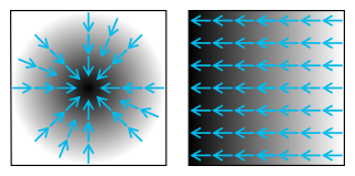
In vector calculus, the gradient of a scalar-valued differentiable function of several variables is the vector field whose value at a point gives the direction and the rate of fastest increase. The gradient transforms like a vector under change of basis of the space of variables of . If the gradient of a function is non-zero at a point , the direction of the gradient is the direction in which the function increases most quickly from , and the magnitude of the gradient is the rate of increase in that direction, the greatest absolute directional derivative. Further, a point where the gradient is the zero vector is known as a stationary point. The gradient thus plays a fundamental role in optimization theory, where it is used to minimize a function by gradient descent. In coordinate-free terms, the gradient of a function may be defined by:
In mathematics, a spherical coordinate system is a coordinate system for three-dimensional space where the position of a given point in space is specified by three numbers, : the radial distance of the radial liner connecting the point to the fixed point of origin ; the polar angle θ of the radial line r; and the azimuthal angle φ of the radial line r.
In mathematics and physics, Laplace's equation is a second-order partial differential equation named after Pierre-Simon Laplace, who first studied its properties. This is often written as
In mathematical analysis, the Dirac delta function, also known as the unit impulse, is a generalized function on the real numbers, whose value is zero everywhere except at zero, and whose integral over the entire real line is equal to one. Since there is no function having this property, to model the delta "function" rigorously involves the use of limits or, as is common in mathematics, measure theory and the theory of distributions.
A Fourier series is an expansion of a periodic function into a sum of trigonometric functions. The Fourier series is an example of a trigonometric series, but not all trigonometric series are Fourier series. By expressing a function as a sum of sines and cosines, many problems involving the function become easier to analyze because trigonometric functions are well understood. For example, Fourier series were first used by Joseph Fourier to find solutions to the heat equation. This application is possible because the derivatives of trigonometric functions fall into simple patterns. Fourier series cannot be used to approximate arbitrary functions, because most functions have infinitely many terms in their Fourier series, and the series do not always converge. Well-behaved functions, for example smooth functions, have Fourier series that converge to the original function. The coefficients of the Fourier series are determined by integrals of the function multiplied by trigonometric functions, described in Common forms of the Fourier series below.
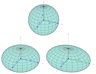
An ellipsoid is a surface that can be obtained from a sphere by deforming it by means of directional scalings, or more generally, of an affine transformation.
In mathematics, a unit vector in a normed vector space is a vector of length 1. A unit vector is often denoted by a lowercase letter with a circumflex, or "hat", as in .
In mathematics, the Laplace operator or Laplacian is a differential operator given by the divergence of the gradient of a scalar function on Euclidean space. It is usually denoted by the symbols , (where is the nabla operator), or . In a Cartesian coordinate system, the Laplacian is given by the sum of second partial derivatives of the function with respect to each independent variable. In other coordinate systems, such as cylindrical and spherical coordinates, the Laplacian also has a useful form. Informally, the Laplacian Δf (p) of a function f at a point p measures by how much the average value of f over small spheres or balls centered at p deviates from f (p).
Unit quaternions, known as versors, provide a convenient mathematical notation for representing spatial orientations and rotations of elements in three dimensional space. Specifically, they encode information about an axis-angle rotation about an arbitrary axis. Rotation and orientation quaternions have applications in computer graphics, computer vision, robotics, navigation, molecular dynamics, flight dynamics, orbital mechanics of satellites, and crystallographic texture analysis.
In vector calculus, the Jacobian matrix of a vector-valued function of several variables is the matrix of all its first-order partial derivatives. When this matrix is square, that is, when the function takes the same number of variables as input as the number of vector components of its output, its determinant is referred to as the Jacobian determinant. Both the matrix and the determinant are often referred to simply as the Jacobian in literature.
In the mathematical field of differential geometry, a metric tensor is an additional structure on a manifold M that allows defining distances and angles, just as the inner product on a Euclidean space allows defining distances and angles there. More precisely, a metric tensor at a point p of M is a bilinear form defined on the tangent space at p, and a metric field on M consists of a metric tensor at each point p of M that varies smoothly with p.
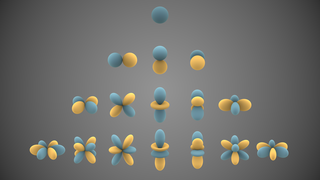
In mathematics and physical science, spherical harmonics are special functions defined on the surface of a sphere. They are often employed in solving partial differential equations in many scientific fields. A list of the spherical harmonics is available in Table of spherical harmonics.
In mathematics, the Radon transform is the integral transform which takes a function f defined on the plane to a function Rf defined on the (two-dimensional) space of lines in the plane, whose value at a particular line is equal to the line integral of the function over that line. The transform was introduced in 1917 by Johann Radon, who also provided a formula for the inverse transform. Radon further included formulas for the transform in three dimensions, in which the integral is taken over planes. It was later generalized to higher-dimensional Euclidean spaces and more broadly in the context of integral geometry. The complex analogue of the Radon transform is known as the Penrose transform. The Radon transform is widely applicable to tomography, the creation of an image from the projection data associated with cross-sectional scans of an object.
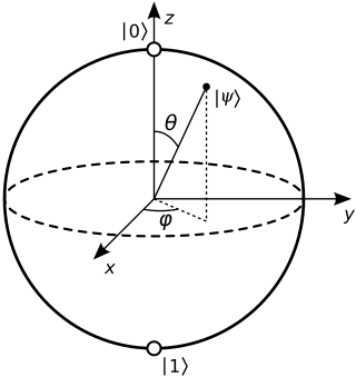
In quantum mechanics and computing, the Bloch sphere is a geometrical representation of the pure state space of a two-level quantum mechanical system (qubit), named after the physicist Felix Bloch.
In mathematics and physics, the Christoffel symbols are an array of numbers describing a metric connection. The metric connection is a specialization of the affine connection to surfaces or other manifolds endowed with a metric, allowing distances to be measured on that surface. In differential geometry, an affine connection can be defined without reference to a metric, and many additional concepts follow: parallel transport, covariant derivatives, geodesics, etc. also do not require the concept of a metric. However, when a metric is available, these concepts can be directly tied to the "shape" of the manifold itself; that shape is determined by how the tangent space is attached to the cotangent space by the metric tensor. Abstractly, one would say that the manifold has an associated (orthonormal) frame bundle, with each "frame" being a possible choice of a coordinate frame. An invariant metric implies that the structure group of the frame bundle is the orthogonal group O(p, q). As a result, such a manifold is necessarily a (pseudo-)Riemannian manifold. The Christoffel symbols provide a concrete representation of the connection of (pseudo-)Riemannian geometry in terms of coordinates on the manifold. Additional concepts, such as parallel transport, geodesics, etc. can then be expressed in terms of Christoffel symbols.
In mathematics (specifically multivariable calculus), a multiple integral is a definite integral of a function of several real variables, for instance, f(x, y) or f(x, y, z). Physical (natural philosophy) interpretation: S any surface, V any volume, etc.. Incl. variable to time, position, etc.
In geometry, various formalisms exist to express a rotation in three dimensions as a mathematical transformation. In physics, this concept is applied to classical mechanics where rotational kinematics is the science of quantitative description of a purely rotational motion. The orientation of an object at a given instant is described with the same tools, as it is defined as an imaginary rotation from a reference placement in space, rather than an actually observed rotation from a previous placement in space.
In fluid dynamics, the Oseen equations describe the flow of a viscous and incompressible fluid at small Reynolds numbers, as formulated by Carl Wilhelm Oseen in 1910. Oseen flow is an improved description of these flows, as compared to Stokes flow, with the (partial) inclusion of convective acceleration.
In geometry, a ball is a region in a space comprising all points within a fixed distance, called the radius, from a given point; that is, it is the region enclosed by a sphere or hypersphere. An n-ball is a ball in an n-dimensional Euclidean space. The volume of a n-ball is the Lebesgue measure of this ball, which generalizes to any dimension the usual volume of a ball in 3-dimensional space. The volume of a n-ball of radius R is where is the volume of the unit n-ball, the n-ball of radius 1.
In the mathematical study of rotational symmetry, the zonal spherical harmonics are special spherical harmonics that are invariant under the rotation through a particular fixed axis. The zonal spherical functions are a broad extension of the notion of zonal spherical harmonics to allow for a more general symmetry group.
Weeks, Jeffrey R. (1985). The Shape of Space: how to visualize surfaces and three-dimensional manifolds. Marcel Dekker. ISBN978-0-8247-7437-0(Chapter 14: The Hypersphere).{{cite book}}: CS1 maint: postscript (link)
This page is based on this Wikipedia article Text is available under the CC BY-SA 4.0 license; additional terms may apply. Images, videos and audio are available under their respective licenses.