Noncentral hypergeometric distributions

Last updated

In statistics, the hypergeometric distribution is the discrete probability distribution generated by picking colored balls at random from an urn without replacement.

Contents

Various generalizations to this distribution exist for cases where the picking of colored balls is biased so that balls of one color are more likely to be picked than balls of another color.

This can be illustrated by the following example. Assume that an opinion poll is conducted by calling random telephone numbers. Unemployed people are more likely to be home and answer the phone than employed people are. Therefore, unemployed respondents are likely to be over-represented in the sample. The probability distribution of employed versus unemployed respondents in a sample of n respondents can be described as a noncentral hypergeometric distribution.

The description of biased urn models is complicated by the fact that there is more than one noncentral hypergeometric distribution. Which distribution one gets depends on whether items (e.g., colored balls) are sampled one by one in a manner in which there is competition between the items or they are sampled independently of one another. The name noncentral hypergeometric distribution has been used for both of these cases. The use of the same name for two different distributions came about because they were studied by two different groups of scientists with hardly any contact with each other.

Agner Fog (2007, 2008) suggested that the best way to avoid confusion is to use the name Wallenius' noncentral hypergeometric distribution for the distribution of a biased urn model in which a predetermined number of items are drawn one by one in a competitive manner and to use the name Fisher's noncentral hypergeometric distribution for one in which items are drawn independently of each other, so that the total number of items drawn is known only after the experiment. The names refer to Kenneth Ted Wallenius and R. A. Fisher, who were the first to describe the respective distributions.

Fisher's noncentral hypergeometric distribution had previously been given the name extended hypergeometric distribution, but this name is rarely used in the scientific literature, except in handbooks that need to distinguish between the two distributions.

Wallenius' noncentral hypergeometric distribution

Wallenius' distribution can be explained as follows. Assume that an urn contains red balls and white balls, totalling balls. balls are drawn at random from the urn one by one without replacement. Each red ball has the weight , and each white ball has the weight . We assume that the probability of taking a particular ball is proportional to its weight. The physical property that determines the odds may be something else than weight, such as size or slipperiness or some other factor, but it is convenient to use the word weight for the odds parameter.

The probability that the first ball picked is red is equal to the weight fraction of red balls:

The probability that the second ball picked is red depends on whether the first ball was red or white. If the first ball was red then the above formula is used with reduced by one. If the first ball was white then the above formula is used with reduced by one.

The important fact that distinguishes Wallenius' distribution is that there is competition between the balls. The probability that a particular ball is taken in a particular draw depends not only on its own weight, but also on the total weight of the competing balls that remain in the urn at that moment. And the weight of the competing balls depends on the outcomes of all preceding draws.

A multivariate version of Wallenius' distribution is used if there are more than two different colors.

The distribution of the balls that are not drawn is a complementary Wallenius' noncentral hypergeometric distribution.

Fisher's noncentral hypergeometric distribution

In the Fisher model, the fates of the balls are independent and there is no dependence between draws. One may as well take all n balls at the same time. Each ball has no "knowledge" of what happens to the other balls. For the same reason, it is impossible to know the value of n before the experiment. If we tried to fix the value of n then we would have no way of preventing ball number n + 1 from being taken without violating the principle of independence between balls. n is therefore a random variable, and the Fisher distribution is a conditional distribution which can only be determined after the experiment when n is observed. The unconditional distribution is two independent binomials, one for each color.

Fisher's distribution can simply be defined as the conditional distribution of two or more independent binomial variates dependent upon their sum. A multivariate version of the Fisher's distribution is used if there are more than two colors of balls.

The difference between the two noncentral hypergeometric distributions

Comparison of distributions with same odds:
Blue: Wallenius o = 0.5
Red: Fisher o = 0.5
Green: Central hypergeometric o = 1.
m1 = 80, m2 = 60, n = 100 NoncentralHypergeometricCompare1.png
Comparison of distributions with same odds:
Blue: Wallenius ω = 0.5
Red: Fisher ω = 0.5
Green: Central hypergeometric ω = 1.
m1 = 80, m2 = 60, n = 100
Comparison of distributions with same mean:
Blue: Wallenius o = 0.5
Red: Fisher o = 0.28
Green: Central hypergeometric o = 1.
m1 = 80, m2 = 60, n = 100 NoncentralHypergeometricCompare2.png
Comparison of distributions with same mean:
Blue: Wallenius ω = 0.5
Red: Fisher ω = 0.28
Green: Central hypergeometric ω = 1.
m1 = 80, m2 = 60, n = 100

Wallenius' and Fisher's distributions are approximately equal when the odds ratio is near 1, and n is low compared to the total number of balls, N. The difference between the two distributions becomes higher when the odds ratio is far from one and n is near N. The two distributions approximate each other better when they have the same mean than when they have the same odds (ω = 1) (see figures above).

Both distributions degenerate into the hypergeometric distribution when the odds ratio is 1, or to the binomial distribution when n = 1.

To understand why the two distributions are different, we may consider the following extreme example: An urn contains one red ball with the weight 1000, and a thousand white balls each with the weight 1. We want to calculate the probability that the red ball is not taken.

First we consider the Wallenius model. The probability that the red ball is not taken in the first draw is 1000/2000 = 12. The probability that the red ball is not taken in the second draw, under the condition that it was not taken in the first draw, is 999/1999 ≈ 12. The probability that the red ball is not taken in the third draw, under the condition that it was not taken in the first two draws, is 998/1998 ≈ 12. Continuing in this way, we can calculate that the probability of not taking the red ball in n draws is approximately 2n as long as n is small compared to N. In other words, the probability of not taking a very heavy ball in n draws falls almost exponentially with n in Wallenius' model. The exponential function arises because the probabilities for each draw are all multiplied together.

This is not the case in Fisher's model, where balls are taken independently, and possibly simultaneously. Here the draws are independent and the probabilities are therefore not multiplied together. The probability of not taking the heavy red ball in Fisher's model is approximately 1/(n + 1). The two distributions are therefore very different in this extreme case, even though they are quite similar in less extreme cases.

The following conditions must be fulfilled for Wallenius' distribution to be applicable:

The following conditions must be fulfilled for Fisher's distribution to be applicable:

Examples

The following examples illustrate which distribution applies in different situations.

Example 1

You are catching fish in a small lake that contains a limited number of fish. There are different kinds of fish with different weights. The probability of catching a particular fish at a particular moment is proportional to its weight.

You are catching the fish one by one with a fishing rod. You have decided to catch n fish. You are determined to catch exactly n fish regardless of how long it may take. You will stop after you have caught n fish even if you can see more fish that are tempting.

This scenario will give a distribution of the types of fish caught that is equal to Wallenius' noncentral hypergeometric distribution.

Example 2

You are catching fish as in example 1, but using a big net. You set up the net one day and come back the next day to remove the net. You count how many fish you have caught and then you go home regardless of how many fish you have caught. Each fish has a probability of being ensnared that is proportional to its weight but independent of what happens to the other fish.

The total number of fish that will be caught in this scenario is not known in advance. The expected number of fish caught is therefore described by multiple binomial distributions, one for each kind of fish.

After the fish have been counted, the total number n of fish is known. The probability distribution when n is known (but the number of each type is not known yet) is Fisher's noncentral hypergeometric distribution.

Example 3

You are catching fish with a small net. It is possible that more than one fish can be caught in the net at the same time. You will use the net repeatedly until you have got at least n fish.

This scenario gives a distribution that lies between Wallenius' and Fisher's distributions. The total number of fish caught can vary if you are getting too many fish in the last catch. You may put the excess fish back into the lake, but this still does not give Wallenius' distribution. This is because you are catching multiple fish at the same time. The condition that each catch depends on all previous catches does not hold for fish that are caught simultaneously or in the same operation.

The resulting distribution will be close to Wallenius' distribution if there are few fish in the net in each catch and many casts of the net. The resulting distribution will be close to Fisher's distribution if there are many fish in the net in each catch and few casts.

Example 4

You are catching fish with a big net. Fish swim into the net randomly in a situation that resembles a Poisson process. You watch the net and take it up as soon as you have caught exactly n fish.

The resulting distribution will be close to Fisher's distribution because the fish arrive in the net independently of each other. But the fates of the fish are not completely independent because a particular fish can be saved from being caught if n other fish happen to arrive in the net before this particular fish. This is more likely to happen if the other fish are heavy than if they are light.

Example 5

You are catching fish one by one with a fishing rod as in example 1. You need a particular amount of fish in order to feed your family. You will stop when the total weight of the fish caught reaches this predetermined limit. The resulting distribution will be close to Wallenius' distribution, but not exactly equal to it because the decision to stop depends on the weight of the fish caught so far. n is therefore not known before the fishing trip.

Conclusion to the examples

These examples show that the distribution of the types of fish caught depends on the way they are caught. Many situations will give a distribution that lies somewhere between Wallenius' and Fisher's noncentral hypergeometric distributions.

A consequence of the difference between these two distributions is that one will catch more of the heavy fish, on average, by catching n fish one by one than by catching all n at the same time. In general, we can say that, in biased sampling, the odds parameter has a stronger effect in Wallenius' distribution than in Fisher's distribution, especially when n/N is high.

Probability mass function for Wallenius' noncentral hypergeometric distribution for different values of the odds ratio o.
m1 = 80, m2 = 60, n = 100, o = 0.1 ... 20 WalleniusNoncentralHypergeometric1.png
Probability mass function for Wallenius' noncentral hypergeometric distribution for different values of the odds ratio ω.
m1 = 80, m2 = 60, n = 100, ω = 0.1 ... 20
Probability mass function for Fisher's noncentral hypergeometric distribution for different values of the odds ratio o.
m1 = 80, m2 = 60, n = 100, o = 0.01 ... 1000 FishersNoncentralHypergeometric1.png
Probability mass function for Fisher's noncentral hypergeometric distribution for different values of the odds ratio ω.
m1 = 80, m2 = 60, n = 100, ω = 0.01 ... 1000

See also

Related Research Articles

<span class="mw-page-title-main">Probability distribution</span> Mathematical function for the probability a given outcome occurs in an experiment

In probability theory and statistics, a probability distribution is the mathematical function that gives the probabilities of occurrence of different possible outcomes for an experiment. It is a mathematical description of a random phenomenon in terms of its sample space and the probabilities of events.

<span class="mw-page-title-main">Random variable</span> Variable representing a random phenomenon

A random variable is a mathematical formalization of a quantity or object which depends on random events. The term 'random variable' can be misleading as its mathematical definition is not actually random nor a variable, but rather it is a function from possible outcomes in a sample space to a measurable space, often to the real numbers.

<span class="mw-page-title-main">Hypergeometric distribution</span> Discrete probability distribution

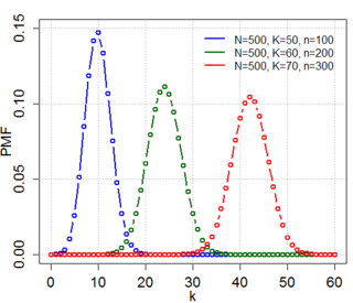
In probability theory and statistics, the hypergeometric distribution is a discrete probability distribution that describes the probability of successes in draws, without replacement, from a finite population of size that contains exactly objects with that feature, wherein each draw is either a success or a failure. In contrast, the binomial distribution describes the probability of successes in draws with replacement.

<span class="mw-page-title-main">Markov property</span> Memoryless property of a stochastic process

In probability theory and statistics, the term Markov property refers to the memoryless property of a stochastic process, which means that its future evolution is independent of its history. It is named after the Russian mathematician Andrey Markov. The term strong Markov property is similar to the Markov property, except that the meaning of "present" is defined in terms of a random variable known as a stopping time.

<span class="mw-page-title-main">Urn problem</span> Mental exercise in probability and statistics

In probability and statistics, an urn problem is an idealized mental exercise in which some objects of real interest are represented as colored balls in an urn or other container. One pretends to remove one or more balls from the urn; the goal is to determine the probability of drawing one color or another, or some other properties. A number of important variations are described below.

Fisher's exact test is a statistical significance test used in the analysis of contingency tables. Although in practice it is employed when sample sizes are small, it is valid for all sample sizes. It is named after its inventor, Ronald Fisher, and is one of a class of exact tests, so called because the significance of the deviation from a null hypothesis can be calculated exactly, rather than relying on an approximation that becomes exact in the limit as the sample size grows to infinity, as with many statistical tests.

<span class="mw-page-title-main">Joint probability distribution</span> Type of probability distribution

Given two random variables that are defined on the same probability space, the joint probability distribution is the corresponding probability distribution on all possible pairs of outputs. The joint distribution can just as well be considered for any given number of random variables. The joint distribution encodes the marginal distributions, i.e. the distributions of each of the individual random variables and the conditional probability distributions, which deal with how the outputs of one random variable are distributed when given information on the outputs of the other random variable(s).

In the field of information retrieval, divergence from randomness, one of the first models, is one type of probabilistic model. It is basically used to test the amount of information carried in the documents. It is based on Harter's 2-Poisson indexing-model. The 2-Poisson model has a hypothesis that the level of the documents is related to a set of documents which contains words occur relatively greater than the rest of the documents. It is not a 'model', but a framework for weighting terms using probabilistic methods, and it has a special relationship for term weighting based on notion of eliteness.

In mathematics, the Kolmogorov extension theorem is a theorem that guarantees that a suitably "consistent" collection of finite-dimensional distributions will define a stochastic process. It is credited to the English mathematician Percy John Daniell and the Russian mathematician Andrey Nikolaevich Kolmogorov.

<span class="mw-page-title-main">Beta-binomial distribution</span> Discrete probability distribution

In probability theory and statistics, the beta-binomial distribution is a family of discrete probability distributions on a finite support of non-negative integers arising when the probability of success in each of a fixed or known number of Bernoulli trials is either unknown or random. The beta-binomial distribution is the binomial distribution in which the probability of success at each of n trials is not fixed but randomly drawn from a beta distribution. It is frequently used in Bayesian statistics, empirical Bayes methods and classical statistics to capture overdispersion in binomial type distributed data.

<span class="mw-page-title-main">Wallenius' noncentral hypergeometric distribution</span>

In probability theory and statistics, Wallenius' noncentral hypergeometric distribution is a generalization of the hypergeometric distribution where items are sampled with bias.

<span class="mw-page-title-main">Fisher's noncentral hypergeometric distribution</span>

In probability theory and statistics, Fisher's noncentral hypergeometric distribution is a generalization of the hypergeometric distribution where sampling probabilities are modified by weight factors. It can also be defined as the conditional distribution of two or more binomially distributed variables dependent upon their fixed sum.

Subjective logic is a type of probabilistic logic that explicitly takes epistemic uncertainty and source trust into account. In general, subjective logic is suitable for modeling and analysing situations involving uncertainty and relatively unreliable sources. For example, it can be used for modeling and analysing trust networks and Bayesian networks.

In probability theory, the chain rule describes how to calculate the probability of the intersection of, not necessarily independent, events or the joint distribution of random variables respectively, using conditional probabilities. The rule is notably used in the context of discrete stochastic processes and in applications, e.g. the study of Bayesian networks, which describe a probability distribution in terms of conditional probabilities.

In statistics, a Pólya urn model, named after George Pólya, is a family of urn models that can be used to interpret many commonly used statistical models.

In probability theory, a beta negative binomial distribution is the probability distribution of a discrete random variable  equal to the number of failures needed to get successes in a sequence of independent Bernoulli trials. The probability of success on each trial stays constant within any given experiment but varies across different experiments following a beta distribution. Thus the distribution is a compound probability distribution.

In mathematics, a statistical manifold is a Riemannian manifold, each of whose points is a probability distribution. Statistical manifolds provide a setting for the field of information geometry. The Fisher information metric provides a metric on these manifolds. Following this definition, the log-likelihood function is a differentiable map and the score is an inclusion.

<span class="mw-page-title-main">Negative hypergeometric distribution</span>

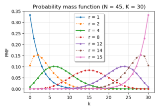
In probability theory and statistics, the negative hypergeometric distribution describes probabilities for when sampling from a finite population without replacement in which each sample can be classified into two mutually exclusive categories like Pass/Fail or Employed/Unemployed. As random selections are made from the population, each subsequent draw decreases the population causing the probability of success to change with each draw. Unlike the standard hypergeometric distribution, which describes the number of successes in a fixed sample size, in the negative hypergeometric distribution, samples are drawn until failures have been found, and the distribution describes the probability of finding successes in such a sample. In other words, the negative hypergeometric distribution describes the likelihood of successes in a sample with exactly failures.

Bayesian hierarchical modelling is a statistical model written in multiple levels that estimates the parameters of the posterior distribution using the Bayesian method. The sub-models combine to form the hierarchical model, and Bayes' theorem is used to integrate them with the observed data and account for all the uncertainty that is present. The result of this integration is the posterior distribution, also known as the updated probability estimate, as additional evidence on the prior distribution is acquired.

References

Johnson, N. L.; Kemp, A. W.; Kotz, S. (2005), Univariate Discrete Distributions, Hoboken, New Jersey: Wiley and Sons.

McCullagh, P.; Nelder, J. A. (1983), Generalized Linear Models, London: Chapman and Hall.

Fog, Agner (2007), Random number theory .

Fog, Agner (2008), "Calculation Methods for Wallenius' Noncentral Hypergeometric Distribution", Communications in Statistics - Simulation and Computation, vol. 37, no. 2, pp. 258–273, doi:10.1080/03610910701790269, S2CID   9040568 .