However, for statistical theory, it provides an exemplar problem in the context of estimation theory which is both simple to state and for which results cannot be obtained in closed form. It also provides an example where imposing the requirement for unbiased estimation might be seen as just adding inconvenience, with no real benefit.
Motivation
In statistics, the standard deviation of a population of numbers is often estimated from a random sample drawn from the population. This is the sample standard deviation, which is defined by
One way of seeing that this is a biased estimator of the standard deviation of the population is to start from the result that s2 is an unbiased estimator for the variance σ2 of the underlying population if that variance exists and the sample values are drawn independently with replacement. The square root is a nonlinear function, and only linear functions commute with taking the expectation. Since the square root is a strictly concave function, it follows from Jensen's inequality that the square root of the sample variance is an underestimate.
The use of n−1 instead of n in the formula for the sample variance is known as Bessel's correction, which corrects the bias in the estimation of the population variance, and some, but not all of the bias in the estimation of the population standard deviation.
It is not possible to find an estimate of the standard deviation which is unbiased for all population distributions, as the bias depends on the particular distribution. Much of the following relates to estimation assuming a normal distribution.
When the random variable is normally distributed, a minor correction exists to eliminate the bias. To derive the correction, note that for normally distributed X, Cochran's theorem implies that has a chi square distribution with degrees of freedom and thus its square root, has a chi distribution with degrees of freedom. Consequently, calculating the expectation of this last expression and rearranging constants,
where the correction factor is the scale mean of the chi distribution with degrees of freedom, . This depends on the sample size n, and is given as follows:[1]
where Γ(·) is the gamma function. An unbiased estimator of σ can be obtained by dividing by . As grows large it approaches 1, and even for smaller values the correction is minor. The figure shows a plot of versus sample size. The table below gives numerical values of and algebraic expressions for some values of ; more complete tables may be found in most textbooks[citation needed] on statistical quality control.
Sample size
Expression of
Numerical value
2
0.7978845608
3
0.8862269255
4
0.9213177319
5
0.9399856030
6
0.9515328619
7
0.9593687891
8
0.9650304561
9
0.9693106998
10
0.9726592741
100
0.9974779761
1000
0.9997497811
10000
0.9999749978
2k
2k+1
It is important to keep in mind this correction only produces an unbiased estimator for normally and independently distributed X. When this condition is satisfied, another result about s involving is that the standard error of s is[2][3], while the standard error of the unbiased estimator is
Rule of thumb for the normal distribution
If calculation of the function c4(n) appears too difficult, there is a simple rule of thumb[4] to take the estimator
The formula differs from the familiar expression for s2 only by having n − 1.5 instead of n − 1 in the denominator. This expression is only approximate; in fact,
The bias is relatively small: say, for it is equal to 2.3%, and for the bias is already 0.1%.
Other distributions
In cases where statistically independent data are modelled by a parametric family of distributions other than the normal distribution, the population standard deviation will, if it exists, be a function of the parameters of the model. One general approach to estimation would be maximum likelihood. Alternatively, it may be possible to use the Rao–Blackwell theorem as a route to finding a good estimate of the standard deviation. In neither case would the estimates obtained usually be unbiased. Notionally, theoretical adjustments might be obtainable to lead to unbiased estimates but, unlike those for the normal distribution, these would typically depend on the estimated parameters.
If the requirement is simply to reduce the bias of an estimated standard deviation, rather than to eliminate it entirely, then two practical approaches are available, both within the context of resampling. These are jackknifing and bootstrapping. Both can be applied either to parametrically based estimates of the standard deviation or to the sample standard deviation.
For non-normal distributions an approximate (up to O(n−1) terms) formula for the unbiased estimator of the standard deviation is
where γ2 denotes the population excess kurtosis. The excess kurtosis may be either known beforehand for certain distributions, or estimated from the data.
Effect of autocorrelation (serial correlation)
The material above, to stress the point again, applies only to independent data. However, real-world data often does not meet this requirement; it is autocorrelated (also known as serial correlation). As one example, the successive readings of a measurement instrument that incorporates some form of “smoothing” (more correctly, low-pass filtering) process will be autocorrelated, since any particular value is calculated from some combination of the earlier and later readings.
Estimates of the variance, and standard deviation, of autocorrelated data will be biased. The expected value of the sample variance is[5]
where n is the sample size (number of measurements) and is the autocorrelation function (ACF) of the data. (Note that the expression in the brackets is simply one minus the average expected autocorrelation for the readings.) If the ACF consists of positive values then the estimate of the variance (and its square root, the standard deviation) will be biased low. That is, the actual variability of the data will be greater than that indicated by an uncorrected variance or standard deviation calculation. It is essential to recognize that, if this expression is to be used to correct for the bias, by dividing the estimate by the quantity in brackets above, then the ACF must be known analytically, not via estimation from the data. This is because the estimated ACF will itself be biased.[6]
Example of bias in standard deviation
To illustrate the magnitude of the bias in the standard deviation, consider a dataset that consists of sequential readings from an instrument that uses a specific digital filter whose ACF is known to be given by
where α is the parameter of the filter, and it takes values from zero to unity. Thus the ACF is positive and geometrically decreasing.
Bias in standard deviation for autocorrelated data.
The figure shows the ratio of the estimated standard deviation to its known value (which can be calculated analytically for this digital filter), for several settings of α as a function of sample size n. Changing α alters the variance reduction ratio of the filter, which is known to be
so that smaller values of α result in more variance reduction, or “smoothing.” The bias is indicated by values on the vertical axis different from unity; that is, if there were no bias, the ratio of the estimated to known standard deviation would be unity. Clearly, for modest sample sizes there can be significant bias (a factor of two, or more).
Variance of the mean
It is often of interest to estimate the variance or standard deviation of an estimated mean rather than the variance of a population. When the data are autocorrelated, this has a direct effect on the theoretical variance of the sample mean, which is[7]
The variance of the sample mean can then be estimated by substituting an estimate of σ2. One such estimate can be obtained from the equation for E[s2] given above. First define the following constants, assuming, again, a known ACF:
so that
This says that the expected value of the quantity obtained by dividing the observed sample variance by the correction factor gives an unbiased estimate of the variance. Similarly, re-writing the expression above for the variance of the mean,
which is an unbiased estimator of the variance of the mean in terms of the observed sample variance and known quantities. If the autocorrelations are identically zero, this expression reduces to the well-known result for the variance of the mean for independent data. The effect of the expectation operator in these expressions is that the equality holds in the mean (i.e., on average).
Estimating the standard deviation of the population
Having the expressions above involving the variance of the population, and of an estimate of the mean of that population, it would seem logical to simply take the square root of these expressions to obtain unbiased estimates of the respective standard deviations. However it is the case that, since expectations are integrals,
Instead, assume a function θ exists such that an unbiased estimator of the standard deviation can be written
and θ depends on the sample size n and the ACF. In the case of NID (normally and independently distributed) data, the radicand is unity and θ is just the c4 function given in the first section above. As with c4, θ approaches unity as the sample size increases (as does γ1).
It can be demonstrated via simulation modeling that ignoring θ (that is, taking it to be unity) and using
removes all but a few percent of the bias caused by autocorrelation, making this a reduced-bias estimator, rather than an unbiased estimator. In practical measurement situations, this reduction in bias can be significant, and useful, even if some relatively small bias remains. The figure above, showing an example of the bias in the standard deviation vs. sample size, is based on this approximation; the actual bias would be somewhat larger than indicated in those graphs since the transformation bias θ is not included there.
Estimating the standard deviation of the sample mean
The unbiased variance of the mean in terms of the population variance and the ACF is given by
and since there are no expected values here, in this case the square root can be taken, so that
Using the unbiased estimate expression above for σ, an estimate of the standard deviation of the mean will then be
If the data are NID, so that the ACF vanishes, this reduces to
In the presence of a nonzero ACF, ignoring the function θ as before leads to the reduced-bias estimator
which again can be demonstrated to remove a useful majority of the bias.
In probability theory and statistics, kurtosis is a measure of the "tailedness" of the probability distribution of a real-valued random variable. Like skewness, kurtosis describes a particular aspect of a probability distribution. There are different ways to quantify kurtosis for a theoretical distribution, and there are corresponding ways of estimating it using a sample from a population. Different measures of kurtosis may have different interpretations.
In probability theory and statistics, a normal distribution or Gaussian distribution is a type of continuous probability distribution for a real-valued random variable. The general form of its probability density function is
In statistics, the standard deviation is a measure of the amount of variation of a random variable expected about its mean. A low standard deviation indicates that the values tend to be close to the mean of the set, while a high standard deviation indicates that the values are spread out over a wider range. The standard deviation is commonly used in the determination of what constitutes an outlier and what does not.
In probability theory and statistics, skewness is a measure of the asymmetry of the probability distribution of a real-valued random variable about its mean. The skewness value can be positive, zero, negative, or undefined.
In probability theory and statistics, variance is the expected value of the squared deviation from the mean of a random variable. The standard deviation (SD) is obtained as the square root of the variance. Variance is a measure of dispersion, meaning it is a measure of how far a set of numbers is spread out from their average value. It is the second central moment of a distribution, and the covariance of the random variable with itself, and it is often represented by , , , , or .
The weighted arithmetic mean is similar to an ordinary arithmetic mean, except that instead of each of the data points contributing equally to the final average, some data points contribute more than others. The notion of weighted mean plays a role in descriptive statistics and also occurs in a more general form in several other areas of mathematics.
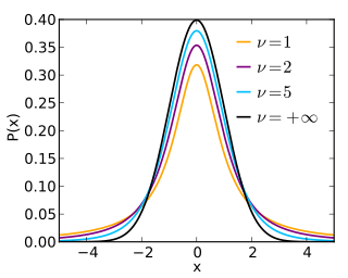
In probability and statistics, Student's t distribution is a continuous probability distribution that generalizes the standard normal distribution. Like the latter, it is symmetric around zero and bell-shaped.
In statistics, the mean squared error (MSE) or mean squared deviation (MSD) of an estimator measures the average of the squares of the errors—that is, the average squared difference between the estimated values and the actual value. MSE is a risk function, corresponding to the expected value of the squared error loss. The fact that MSE is almost always strictly positive is because of randomness or because the estimator does not account for information that could produce a more accurate estimate. In machine learning, specifically empirical risk minimization, MSE may refer to the empirical risk, as an estimate of the true MSE.
In probability theory and statistics, the Rayleigh distribution is a continuous probability distribution for nonnegative-valued random variables. Up to rescaling, it coincides with the chi distribution with two degrees of freedom. The distribution is named after Lord Rayleigh.
In statistics, an effect size is a value measuring the strength of the relationship between two variables in a population, or a sample-based estimate of that quantity. It can refer to the value of a statistic calculated from a sample of data, the value of a parameter for a hypothetical population, or to the equation that operationalizes how statistics or parameters lead to the effect size value. Examples of effect sizes include the correlation between two variables, the regression coefficient in a regression, the mean difference, or the risk of a particular event happening. Effect sizes complement statistical hypothesis testing, and play an important role in power analyses, sample size planning, and in meta-analyses. The cluster of data-analysis methods concerning effect sizes is referred to as estimation statistics.
In statistical inference, specifically predictive inference, a prediction interval is an estimate of an interval in which a future observation will fall, with a certain probability, given what has already been observed. Prediction intervals are often used in regression analysis.
The standard error (SE) of a statistic is the standard deviation of its sampling distribution or an estimate of that standard deviation. If the statistic is the sample mean, it is called the standard error of the mean (SEM). The standard error is a key ingredient in producing confidence intervals.
Directional statistics is the subdiscipline of statistics that deals with directions, axes or rotations in Rn. More generally, directional statistics deals with observations on compact Riemannian manifolds including the Stiefel manifold.
In statistics, a consistent estimator or asymptotically consistent estimator is an estimator—a rule for computing estimates of a parameter θ0—having the property that as the number of data points used increases indefinitely, the resulting sequence of estimates converges in probability to θ0. This means that the distributions of the estimates become more and more concentrated near the true value of the parameter being estimated, so that the probability of the estimator being arbitrarily close to θ0 converges to one.
Estimation theory is a branch of statistics that deals with estimating the values of parameters based on measured empirical data that has a random component. The parameters describe an underlying physical setting in such a way that their value affects the distribution of the measured data. An estimator attempts to approximate the unknown parameters using the measurements. In estimation theory, two approaches are generally considered:
In statistics, simple linear regression (SLR) is a linear regression model with a single explanatory variable. That is, it concerns two-dimensional sample points with one independent variable and one dependent variable and finds a linear function that, as accurately as possible, predicts the dependent variable values as a function of the independent variable. The adjective simple refers to the fact that the outcome variable is related to a single predictor.
In statistics, the bias of an estimator is the difference between this estimator's expected value and the true value of the parameter being estimated. An estimator or decision rule with zero bias is called unbiased. In statistics, "bias" is an objective property of an estimator. Bias is a distinct concept from consistency: consistent estimators converge in probability to the true value of the parameter, but may be biased or unbiased; see bias versus consistency for more.
In statistics, pooled variance is a method for estimating variance of several different populations when the mean of each population may be different, but one may assume that the variance of each population is the same. The numerical estimate resulting from the use of this method is also called the pooled variance.
In statistics, Bessel's correction is the use of n − 1 instead of n in the formula for the sample variance and sample standard deviation, where n is the number of observations in a sample. This method corrects the bias in the estimation of the population variance. It also partially corrects the bias in the estimation of the population standard deviation. However, the correction often increases the mean squared error in these estimations. This technique is named after Friedrich Bessel.
In probability theory and directional statistics, a wrapped normal distribution is a wrapped probability distribution that results from the "wrapping" of the normal distribution around the unit circle. It finds application in the theory of Brownian motion and is a solution to the heat equation for periodic boundary conditions. It is closely approximated by the von Mises distribution, which, due to its mathematical simplicity and tractability, is the most commonly used distribution in directional statistics.
References
↑ Ben W. Bolch, "More on unbiased estimation of the standard deviation", The American Statistician, 22(3), p. 27 (1968)
↑ Duncan, A. J., Quality Control and Industrial Statistics 4th Ed., Irwin (1974) ISBN0-256-01558-9, p.139
N.L. Johnson, S. Kotz, and N. Balakrishnan, Continuous Univariate Distributions, Volume 1, 2nd edition, Wiley and sons, 1994. ISBN0-471-58495-9. Chapter 13, Section 8.2
↑ Richard M. Brugger, "A Note on Unbiased Estimation on the Standard Deviation", The American Statistician (23) 4 p. 32 (1969)
↑ Law and Kelton, Simulation Modeling and Analysis, 2nd Ed. McGraw-Hill (1991), p.284, ISBN0-07-036698-5. This expression can be derived from its original source in Anderson, The Statistical Analysis of Time Series, Wiley (1971), ISBN0-471-04745-7, p.448, Equation 51.
↑ Law and Kelton, p.286. This bias is quantified in Anderson, p.448, Equations 52–54.
↑ Law and Kelton, p.285. This equation can be derived from Theorem 8.2.3 of Anderson. It also appears in Box, Jenkins, Reinsel, Time Series Analysis: Forecasting and Control, 4th Ed. Wiley (2008), ISBN978-0-470-27284-8, p.31.
This page is based on this Wikipedia article Text is available under the CC BY-SA 4.0 license; additional terms may apply. Images, videos and audio are available under their respective licenses.