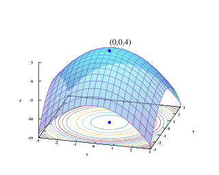
Quadratic programming (QP) is the process of solving certain mathematical optimization problems involving quadratic functions. Specifically, one seeks to optimize a multivariate quadratic function subject to linear constraints on the variables. Quadratic programming is a type of nonlinear programming.

Linear programming (LP), also called linear optimization, is a method to achieve the best outcome in a mathematical model whose requirements and objective are represented by linear relationships. Linear programming is a special case of mathematical programming.
Mathematical optimization or mathematical programming is the selection of a best element, with regard to some criteria, from some set of available alternatives. It is generally divided into two subfields: discrete optimization and continuous optimization. Optimization problems arise in all quantitative disciplines from computer science and engineering to operations research and economics, and the development of solution methods has been of interest in mathematics for centuries.
An integer programming problem is a mathematical optimization or feasibility program in which some or all of the variables are restricted to be integers. In many settings the term refers to integer linear programming (ILP), in which the objective function and the constraints are linear.
In mathematics, the Hessian matrix, Hessian or Hesse matrix is a square matrix of second-order partial derivatives of a scalar-valued function, or scalar field. It describes the local curvature of a function of many variables. The Hessian matrix was developed in the 19th century by the German mathematician Ludwig Otto Hesse and later named after him. Hesse originally used the term "functional determinants". The Hessian is sometimes denoted by H or, ambiguously, by ∇2.
In mathematics, nonlinear programming (NLP) is the process of solving an optimization problem where some of the constraints are not linear equalities or the objective function is not a linear function. An optimization problem is one of calculation of the extrema of an objective function over a set of unknown real variables and conditional to the satisfaction of a system of equalities and inequalities, collectively termed constraints. It is the sub-field of mathematical optimization that deals with problems that are not linear.
In mathematics and computing, the Levenberg–Marquardt algorithm, also known as the damped least-squares (DLS) method, is used to solve non-linear least squares problems. These minimization problems arise especially in least squares curve fitting. The LMA interpolates between the Gauss–Newton algorithm (GNA) and the method of gradient descent. The LMA is more robust than the GNA, which means that in many cases it finds a solution even if it starts very far off the final minimum. For well-behaved functions and reasonable starting parameters, the LMA tends to be slower than the GNA. LMA can also be viewed as Gauss–Newton using a trust region approach.
Convex optimization is a subfield of mathematical optimization that studies the problem of minimizing convex functions over convex sets. Many classes of convex optimization problems admit polynomial-time algorithms, whereas mathematical optimization is in general NP-hard.
In numerical optimization, the Broyden–Fletcher–Goldfarb–Shanno (BFGS) algorithm is an iterative method for solving unconstrained nonlinear optimization problems. Like the related Davidon–Fletcher–Powell method, BFGS determines the descent direction by preconditioning the gradient with curvature information. It does so by gradually improving an approximation to the Hessian matrix of the loss function, obtained only from gradient evaluations via a generalized secant method.
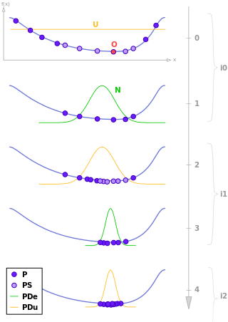
Estimation of distribution algorithms (EDAs), sometimes called probabilistic model-building genetic algorithms (PMBGAs), are stochastic optimization methods that guide the search for the optimum by building and sampling explicit probabilistic models of promising candidate solutions. Optimization is viewed as a series of incremental updates of a probabilistic model, starting with the model encoding an uninformative prior over admissible solutions and ending with the model that generates only the global optima.
In mathematical optimization, constrained optimization is the process of optimizing an objective function with respect to some variables in the presence of constraints on those variables. The objective function is either a cost function or energy function, which is to be minimized, or a reward function or utility function, which is to be maximized. Constraints can be either hard constraints, which set conditions for the variables that are required to be satisfied, or soft constraints, which have some variable values that are penalized in the objective function if, and based on the extent that, the conditions on the variables are not satisfied.
Penalty methods are a certain class of algorithms for solving constrained optimization problems.
Multi-objective optimization or Pareto optimization is an area of multiple-criteria decision making that is concerned with mathematical optimization problems involving more than one objective function to be optimized simultaneously. Multi-objective is a type of vector optimization that has been applied in many fields of science, including engineering, economics and logistics where optimal decisions need to be taken in the presence of trade-offs between two or more conflicting objectives. Minimizing cost while maximizing comfort while buying a car, and maximizing performance whilst minimizing fuel consumption and emission of pollutants of a vehicle are examples of multi-objective optimization problems involving two and three objectives, respectively. In practical problems, there can be more than three objectives.
Phase retrieval is the process of algorithmically finding solutions to the phase problem. Given a complex spectrum , of amplitude , and phase :
In mathematical optimization, the firefly algorithm is a metaheuristic proposed by Xin-She Yang and inspired by the flashing behavior of fireflies.
In operations research, cuckoo search is an optimization algorithm developed by Xin-She Yang and Suash Deb in 2009. It has been shown to be a special case of the well-known -evolution strategy. It was inspired by the obligate brood parasitism of some cuckoo species by laying their eggs in the nests of host birds of other species. Some host birds can engage direct conflict with the intruding cuckoos. For example, if a host bird discovers the eggs are not their own, it will either throw these alien eggs away or simply abandon its nest and build a new nest elsewhere. Some cuckoo species such as the New World brood-parasitic Tapera have evolved in such a way that female parasitic cuckoos are often very specialized in the mimicry in colors and pattern of the eggs of a few chosen host species. Cuckoo search idealized such breeding behavior, and thus can be applied for various optimization problems.
In mathematics, a submodular set function is a set function that, informally, describes the relationship between a set of inputs and an output, where adding more of one input has a decreasing additional benefit. The natural diminishing returns property which makes them suitable for many applications, including approximation algorithms, game theory and electrical networks. Recently, submodular functions have also found utility in several real world problems in machine learning and artificial intelligence, including automatic summarization, multi-document summarization, feature selection, active learning, sensor placement, image collection summarization and many other domains.
Quantum optimization algorithms are quantum algorithms that are used to solve optimization problems. Mathematical optimization deals with finding the best solution to a problem from a set of possible solutions. Mostly, the optimization problem is formulated as a minimization problem, where one tries to minimize an error which depends on the solution: the optimal solution has the minimal error. Different optimization techniques are applied in various fields such as mechanics, economics and engineering, and as the complexity and amount of data involved rise, more efficient ways of solving optimization problems are needed. Quantum computing may allow problems which are not practically feasible on classical computers to be solved, or suggest a considerable speed up with respect to the best known classical algorithm.
In evolutionary computation, Minimum Population Search (MPS) is a computational method that optimizes a problem by iteratively trying to improve a set of candidate solutions with regard to a given measure of quality. It solves a problem by evolving a small population of candidate solutions by means of relatively simple arithmetical operations.

Dispersive flies optimisation (DFO) is a bare-bones swarm intelligence algorithm which is inspired by the swarming behaviour of flies hovering over food sources. DFO is a simple optimiser which works by iteratively trying to improve a candidate solution with regard to a numerical measure that is calculated by a fitness function. Each member of the population, a fly or an agent, holds a candidate solution whose suitability can be evaluated by their fitness value. Optimisation problems are often formulated as either minimisation or maximisation problems.


