Signorini problem

Last updated

The Signorini problem is an elastostatics problem in linear elasticity: it consists in finding the elastic equilibrium configuration of an anisotropic non-homogeneous elastic body, resting on a rigid frictionless surface and subject only to its mass forces. The name was coined by Gaetano Fichera to honour his teacher, Antonio Signorini: the original name coined by him is problem with ambiguous boundary conditions .

Contents

History

The classical Signorini problem: what will be the equilibrium configuration of the orange spherically shaped elastic body resting on the blue rigid frictionless plane? Classical Signorini problem.svg
The classical Signorini problem: what will be the equilibrium configuration of the orange spherically shaped elastic body resting on the blue rigid frictionless plane?
  • -"Il mio discepolo Fichera mi ha dato una grande soddisfazione"
  • -"Ma Lei ne ha avute tante, Professore, durante la Sua vita", rispose il Dottor Aprile, ma Signorini rispose di nuovo:
  • -"Ma questa è la più grande." E queste furono le sue ultime parole. [1]
Gaetano Fichera, (Fichera 1995, p. 49)

The problem was posed by Antonio Signorini during a course taught at the Istituto Nazionale di Alta Matematica in 1959, later published as the article ( Signorini 1959 ), expanding a previous short exposition he gave in a note published in 1933. Signorini (1959 , p. 128) himself called it problem with ambiguous boundary conditions , [2] since there are two alternative sets of boundary conditions the solution must satisfy on any given contact point. The statement of the problem involves not only equalities but also inequalities , and it is not a priori known what of the two sets of boundary conditions is satisfied at each point. Signorini asked to determine if the problem is well-posed or not in a physical sense, i.e. if its solution exists and is unique or not: he explicitly invited young analysts to study the problem. [3]

Gaetano Fichera and Mauro Picone attended the course, and Fichera started to investigate the problem: since he found no references to similar problems in the theory of boundary value problems, [4] he decided to approach it by starting from first principles, specifically from the virtual work principle.

During Fichera's researches on the problem, Signorini began to suffer serious health problems: nevertheless, he desired to know the answer to his question before his death. Picone, being tied by a strong friendship with Signorini, began to chase Fichera to find a solution: Fichera himself, being tied as well to Signorini by similar feelings, perceived the last months of 1962 as worrying days. [5] Finally, on the first days of January 1963, Fichera was able to give a complete proof of the existence of a unique solution for the problem with ambiguous boundary condition, which he called the "Signorini problem" to honour his teacher. A preliminary research announcement, later published as ( Fichera 1963 ), was written up and submitted to Signorini exactly a week before his death. Signorini expressed great satisfaction to see a solution to his question.
A few days later, Signorini had with his family Doctor, Damiano Aprile, the conversation quoted above. [6]

The solution of the Signorini problem coincides with the birth of the field of variational inequalities. [7]

Formal statement of the problem

The content of this section and the following subsections follows closely the treatment of Gaetano Fichera in Fichera 1963, Fichera 1964b and also Fichera 1995: his derivation of the problem is different from Signorini's one in that he does not consider only incompressible bodies and a plane rest surface, as Signorini does. [8] The problem consist in finding the displacement vector from the natural configuration of an anisotropic non-homogeneous elastic body that lies in a subset of the three-dimensional euclidean space whose boundary is and whose interior normal is the vector , resting on a rigid frictionless surface whose contact surface (or more generally contact set) is and subject only to its body forces , and surface forces applied on the free (i.e. not in contact with the rest surface) surface : the set and the contact surface characterize the natural configuration of the body and are known a priori. Therefore, the body has to satisfy the general equilibrium equations

(1)     

written using the Einstein notation as all in the following development, the ordinary boundary conditions on

(2)     

and the following two sets of boundary conditions on , where is the Cauchy stress tensor. Obviously, the body forces and surface forces cannot be given in arbitrary way but they must satisfy a condition in order for the body to reach an equilibrium configuration: this condition will be deduced and analyzed in the following development.

The ambiguous boundary conditions

If is any tangent vector to the contact set , then the ambiguous boundary condition in each point of this set are expressed by the following two systems of inequalities

(3)          or     (4)     

Let's analyze their meaning:

Knowing these facts, the set of conditions (3) applies to points of the boundary of the body which do not leave the contact set in the equilibrium configuration, since, according to the first relation, the displacement vector has no components directed as the normal vector , while, according to the second relation, the tension vector may have a component directed as the normal vector and having the same sense. In an analogous way, the set of conditions (4) applies to points of the boundary of the body which leave that set in the equilibrium configuration, since displacement vector has a component directed as the normal vector , while the tension vector has no components directed as the normal vector . For both sets of conditions, the tension vector has no tangent component to the contact set, according to the hypothesis that the body rests on a rigid frictionless surface.

Each system expresses a unilateral constraint, in the sense that they express the physical impossibility of the elastic body to penetrate into the surface where it rests: the ambiguity is not only in the unknown values non-zero quantities must satisfy on the contact set but also in the fact that it is not a priori known if a point belonging to that set satisfies the system of boundary conditions (3) or (4) . The set of points where (3) is satisfied is called the area of support of the elastic body on , while its complement respect to is called the area of separation.

The above formulation is general since the Cauchy stress tensor i.e. the constitutive equation of the elastic body has not been made explicit: it is equally valid assuming the hypothesis of linear elasticity or the ones of nonlinear elasticity. However, as it would be clear from the following developments, the problem is inherently nonlinear, therefore assuming a linear stress tensor does not simplify the problem.

The form of the stress tensor in the formulation of Signorini and Fichera

The form assumed by Signorini and Fichera for the elastic potential energy is the following one (as in the previous developments, the Einstein notation is adopted)

where

The Cauchy stress tensor has therefore the following form

(5)     

and it is linear with respect to the components of the infinitesimal strain tensor; however, it is not homogeneous nor isotropic.

Solution of the problem

As for the section on the formal statement of the Signorini problem, the contents of this section and the included subsections follow closely the treatment of Gaetano Fichera in Fichera 1963, Fichera 1964b, Fichera 1972 and also Fichera 1995: obviously, the exposition focuses on the basics steps of the proof of the existence and uniqueness for the solution of problem (1) , (2) , (3) , (4) and (5) , rather than the technical details.

The potential energy

The first step of the analysis of Fichera as well as the first step of the analysis of Antonio Signorini in Signorini 1959 is the analysis of the potential energy, i.e. the following functional

(6)      

where belongs to the set of admissible displacements i.e. the set of displacement vectors satisfying the system of boundary conditions (3) or (4) . The meaning of each of the three terms is the following

Signorini (1959 , pp. 129–133) was able to prove that the admissible displacement which minimize the integral is a solution of the problem with ambiguous boundary conditions (1) , (2) , (3) , (4) and (5) , provided it is a function supported on the closure of the set : however Gaetano Fichera gave a class of counterexamples in ( Fichera 1964b , pp. 619–620) showing that in general, admissible displacements are not smooth functions of these class. Therefore, Fichera tries to minimize the functional (6) in a wider function space: in doing so, he first calculates the first variation (or functional derivative) of the given functional in the neighbourhood of the sought minimizing admissible displacement , and then requires it to be greater than or equal to zero

Defining the following functionals

and

the preceding inequality is can be written as

(7)      

This inequality is the variational inequality for the Signorini problem.

See also

Notes

  1. Free English translation:
    • "My disciple Fichera gave me a great contentment".
    • "But you had many, Professor, during your life", replied Doctor Aprile, but then Signorini replied again:
    • "But this is the greatest one". And those were his last words.
  2. Italian : Problema con ambigue condizioni al contorno.
  3. As it is stated in ( Signorini 1959 , p. 129).
  4. See ( Fichera 1995 , p. 49).
  5. This dramatic situation is described by Fichera (1995 , p. 51) himself.
  6. Fichera (1995 , p. 53) reports the episode following the remembrances of Mauro Picone: see the entry "Antonio Signorini" for further details.
  7. According to Antman (1983 , p. 282)
  8. See Signorini 1959 , p. 127) for the original approach.

Related Research Articles

<span class="mw-page-title-main">Navier–Stokes equations</span> Equations describing the motion of viscous fluid substances

The Navier–Stokes equations are partial differential equations which describe the motion of viscous fluid substances, named after French engineer and physicist Claude-Louis Navier and Anglo-Irish physicist and mathematician George Gabriel Stokes. They were developed over several decades of progressively building the theories, from 1822 (Navier) to 1842-1850 (Stokes).

In continuum mechanics, the infinitesimal strain theory is a mathematical approach to the description of the deformation of a solid body in which the displacements of the material particles are assumed to be much smaller than any relevant dimension of the body; so that its geometry and the constitutive properties of the material at each point of space can be assumed to be unchanged by the deformation.

<span class="mw-page-title-main">Hooke's law</span> Physical law: force needed to deform a spring scales linearly with distance

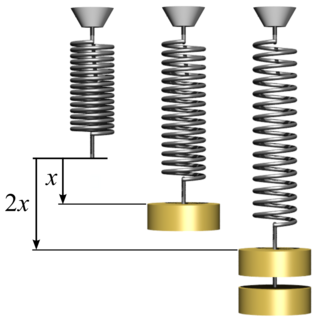
In physics, Hooke's law is an empirical law which states that the force needed to extend or compress a spring by some distance scales linearly with respect to that distance—that is, Fs = kx, where k is a constant factor characteristic of the spring, and x is small compared to the total possible deformation of the spring. The law is named after 17th-century British physicist Robert Hooke. He first stated the law in 1676 as a Latin anagram. He published the solution of his anagram in 1678 as: ut tensio, sic vis. Hooke states in the 1678 work that he was aware of the law since 1660.

In the calculus of variations and classical mechanics, the Euler–Lagrange equations are a system of second-order ordinary differential equations whose solutions are stationary points of the given action functional. The equations were discovered in the 1750s by Swiss mathematician Leonhard Euler and Italian mathematician Joseph-Louis Lagrange.

Linear elasticity is a mathematical model of how solid objects deform and become internally stressed due to prescribed loading conditions. It is a simplification of the more general nonlinear theory of elasticity and a branch of continuum mechanics.

In mathematics, a variational inequality is an inequality involving a functional, which has to be solved for all possible values of a given variable, belonging usually to a convex set. The mathematical theory of variational inequalities was initially developed to deal with equilibrium problems, precisely the Signorini problem: in that model problem, the functional involved was obtained as the first variation of the involved potential energy. Therefore, it has a variational origin, recalled by the name of the general abstract problem. The applicability of the theory has since been expanded to include problems from economics, finance, optimization and game theory.

In statistics, ordinary least squares (OLS) is a type of linear least squares method for choosing the unknown parameters in a linear regression model by the principle of least squares: minimizing the sum of the squares of the differences between the observed dependent variable in the input dataset and the output of the (linear) function of the independent variable.

<span class="mw-page-title-main">Two-state quantum system</span> Simple quantum mechanical system

In quantum mechanics, a two-state system is a quantum system that can exist in any quantum superposition of two independent quantum states. The Hilbert space describing such a system is two-dimensional. Therefore, a complete basis spanning the space will consist of two independent states. Any two-state system can also be seen as a qubit.

<span class="mw-page-title-main">Euler–Bernoulli beam theory</span> Method for load calculation in construction

Euler–Bernoulli beam theory is a simplification of the linear theory of elasticity which provides a means of calculating the load-carrying and deflection characteristics of beams. It covers the case corresponding to small deflections of a beam that is subjected to lateral loads only. By ignoring the effects of shear deformation and rotatory inertia, it is thus a special case of Timoshenko–Ehrenfest beam theory. It was first enunciated circa 1750, but was not applied on a large scale until the development of the Eiffel Tower and the Ferris wheel in the late 19th century. Following these successful demonstrations, it quickly became a cornerstone of engineering and an enabler of the Second Industrial Revolution.

The J-integral represents a way to calculate the strain energy release rate, or work (energy) per unit fracture surface area, in a material. The theoretical concept of J-integral was developed in 1967 by G. P. Cherepanov and independently in 1968 by James R. Rice, who showed that an energetic contour path integral was independent of the path around a crack.

<span class="mw-page-title-main">Hyperelastic material</span>

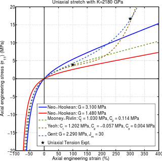
A hyperelastic or Green elastic material is a type of constitutive model for ideally elastic material for which the stress–strain relationship derives from a strain energy density function. The hyperelastic material is a special case of a Cauchy elastic material.

<span class="mw-page-title-main">Mathematical descriptions of the electromagnetic field</span> Formulations of electromagnetism

There are various mathematical descriptions of the electromagnetic field that are used in the study of electromagnetism, one of the four fundamental interactions of nature. In this article, several approaches are discussed, although the equations are in terms of electric and magnetic fields, potentials, and charges with currents, generally speaking.

<span class="mw-page-title-main">Viscoplasticity</span> Theory in continuum mechanics

Viscoplasticity is a theory in continuum mechanics that describes the rate-dependent inelastic behavior of solids. Rate-dependence in this context means that the deformation of the material depends on the rate at which loads are applied. The inelastic behavior that is the subject of viscoplasticity is plastic deformation which means that the material undergoes unrecoverable deformations when a load level is reached. Rate-dependent plasticity is important for transient plasticity calculations. The main difference between rate-independent plastic and viscoplastic material models is that the latter exhibit not only permanent deformations after the application of loads but continue to undergo a creep flow as a function of time under the influence of the applied load.

<span class="mw-page-title-main">Deformation (physics)</span> Transformation of a body from a reference configuration to a current configuration

In physics and continuum mechanics, deformation is the transformation of a body from a reference configuration to a current configuration. A configuration is a set containing the positions of all particles of the body.

The obstacle problem is a classic motivating example in the mathematical study of variational inequalities and free boundary problems. The problem is to find the equilibrium position of an elastic membrane whose boundary is held fixed, and which is constrained to lie above a given obstacle. It is deeply related to the study of minimal surfaces and the capacity of a set in potential theory as well. Applications include the study of fluid filtration in porous media, constrained heating, elasto-plasticity, optimal control, and financial mathematics.

The purpose of this page is to provide supplementary materials for the ordinary least squares article, reducing the load of the main article with mathematics and improving its accessibility, while at the same time retaining the completeness of exposition.

In continuum mechanics, a compatible deformation tensor field in a body is that unique tensor field that is obtained when the body is subjected to a continuous, single-valued, displacement field. Compatibility is the study of the conditions under which such a displacement field can be guaranteed. Compatibility conditions are particular cases of integrability conditions and were first derived for linear elasticity by Barré de Saint-Venant in 1864 and proved rigorously by Beltrami in 1886.

<span class="mw-page-title-main">Kirchhoff–Love plate theory</span>

The Kirchhoff–Love theory of plates is a two-dimensional mathematical model that is used to determine the stresses and deformations in thin plates subjected to forces and moments. This theory is an extension of Euler-Bernoulli beam theory and was developed in 1888 by Love using assumptions proposed by Kirchhoff. The theory assumes that a mid-surface plane can be used to represent a three-dimensional plate in two-dimensional form.

<span class="mw-page-title-main">Rock mass plasticity</span>

Plasticity theory for rocks is concerned with the response of rocks to loads beyond the elastic limit. Historically, conventional wisdom has it that rock is brittle and fails by fracture while plasticity is identified with ductile materials. In field scale rock masses, structural discontinuities exist in the rock indicating that failure has taken place. Since the rock has not fallen apart, contrary to expectation of brittle behavior, clearly elasticity theory is not the last work.

<span class="mw-page-title-main">Flow plasticity theory</span>

Flow plasticity is a solid mechanics theory that is used to describe the plastic behavior of materials. Flow plasticity theories are characterized by the assumption that a flow rule exists that can be used to determine the amount of plastic deformation in the material.

References

Historical references

Research works