Grashof number

Last updated

In fluid mechanics (especially fluid thermodynamics), the Grashof number (Gr, after Franz Grashof [lower-alpha 1] ) is a dimensionless number which approximates the ratio of the buoyancy to viscous forces acting on a fluid. It frequently arises in the study of situations involving natural convection and is analogous to the Reynolds number (Re). [2]

Contents

Definition

Heat transfer

Free convection is caused by a change in density of a fluid due to a temperature change or gradient. Usually the density decreases due to an increase in temperature and causes the fluid to rise. This motion is caused by the buoyancy force. The major force that resists the motion is the viscous force. The Grashof number is a way to quantify the opposing forces. [3]

The Grashof number is:

for vertical flat plates
for pipes
for bluff bodies

where:

The L and D subscripts indicate the length scale basis for the Grashof number.

The transition to turbulent flow occurs in the range 108 < GrL < 109 for natural convection from vertical flat plates. At higher Grashof numbers, the boundary layer is turbulent; at lower Grashof numbers, the boundary layer is laminar, that is, in the range 103 < GrL < 106.

Mass transfer

There is an analogous form of the Grashof number used in cases of natural convection mass transfer problems. In the case of mass transfer, natural convection is caused by concentration gradients rather than temperature gradients. [2]

where

and:

Relationship to other dimensionless numbers

The Rayleigh number, shown below, is a dimensionless number that characterizes convection problems in heat transfer. A critical value exists for the Rayleigh number, above which fluid motion occurs. [3]

The ratio of the Grashof number to the square of the Reynolds number may be used to determine if forced or free convection may be neglected for a system, or if there's a combination of the two. This characteristic ratio is known as the Richardson number (Ri). If the ratio is much less than one, then free convection may be ignored. If the ratio is much greater than one, forced convection may be ignored. Otherwise, the regime is combined forced and free convection. [2]

Derivation

The first step to deriving the Grashof number is manipulating the volume expansion coefficient, as follows.

The in the equation above, which represents specific volume, is not the same as the in the subsequent sections of this derivation, which will represent a velocity. This partial relation of the volume expansion coefficient, , with respect to fluid density, , given constant pressure, can be rewritten as

where:

There are two different ways to find the Grashof number from this point. One involves the energy equation while the other incorporates the buoyant force due to the difference in density between the boundary layer and bulk fluid.

Energy equation

This discussion involving the energy equation is with respect to rotationally symmetric flow. This analysis will take into consideration the effect of gravitational acceleration on flow and heat transfer. The mathematical equations to follow apply both to rotational symmetric flow as well as two-dimensional planar flow.

where:

In this equation the superscript n is to differentiate between rotationally symmetric flow from planar flow. The following characteristics of this equation hold true.

This equation expands to the following with the addition of physical fluid properties:

From here we can further simplify the momentum equation by setting the bulk fluid velocity to 0 ().

This relation shows that the pressure gradient is simply a product of the bulk fluid density and the gravitational acceleration. The next step is to plug in the pressure gradient into the momentum equation.

Further simplification of the momentum equation comes by substituting the volume expansion coefficient, density relationship , found above, and kinematic viscosity relationship, , into the momentum equation.

To find the Grashof number from this point, the preceding equation must be non-dimensionalized. This means that every variable in the equation should have no dimension and should instead be a ratio characteristic to the geometry and setup of the problem. This is done by dividing each variable by corresponding constant quantities. Lengths are divided by a characteristic length, . Velocities are divided by appropriate reference velocities, , which, considering the Reynolds number, gives . Temperatures are divided by the appropriate temperature difference, . These dimensionless parameters look like the following:

The asterisks represent dimensionless parameter. Combining these dimensionless equations with the momentum equations gives the following simplified equation.

where:

is the surface temperature
is the bulk fluid temperature
is the characteristic length.

The dimensionless parameter enclosed in the brackets in the preceding equation is known as the Grashof number:

Buckingham π theorem

Another form of dimensional analysis that will result in the Grashof number is known as the Buckingham π theorem. This method takes into account the buoyancy force per unit volume, due to the density difference in the boundary layer and the bulk fluid.

This equation can be manipulated to give,

The list of variables that are used in the Buckingham π method is listed below, along with their symbols and dimensions.

VariableSymbolDimensions
Significant length
Fluid viscosity
Fluid heat capacity
Fluid thermal conductivity
Volume expansion coefficient
Gravitational acceleration
Temperature difference
Heat transfer coefficient

With reference to the Buckingham π theorem there are 9 – 5 = 4 dimensionless groups. Choose L, k, g and as the reference variables. Thus the groups are as follows:

,
,
,
.

Solving these groups gives:

,
,
,

From the two groups and the product forms the Grashof number:

Taking and the preceding equation can be rendered as the same result from deriving the Grashof number from the energy equation.

In forced convection the Reynolds number governs the fluid flow. But, in natural convection the Grashof number is the dimensionless parameter that governs the fluid flow. Using the energy equation and the buoyant force combined with dimensional analysis provides two different ways to derive the Grashof number.

Physical Reasoning

It is also possible to derive the Grashof number by physical definition of the number as follows:

However, above expression, especially the final part at the right hand side, is slightly different from Grashof number appearing in literature. Following dimensionally correct scale in terms of dynamic viscosity can be used to have the final form.

Writing above scale in Gr gives;

Physical reasoning is helpful to grasp the meaning of the number. On the other hand, following velocity definition can be used as a characteristic velocity value for making certain velocities nondimensional.

Effects of Grashof number on the flow of different fluids

In a recent research carried out on the effects of Grashof number on the flow of different fluids driven by convection over various surfaces. [4] Using slope of the linear regression line through data points, it is concluded that increase in the value of Grashof number or any buoyancy related parameter implies an increase in the wall temperature and this makes the bond(s) between the fluid to become weaker, strength of the internal friction to decrease, the gravity to becomes stronger enough (i.e. makes the specific weight appreciably different between the immediate fluid layers adjacent to the wall). The effects of buoyancy parameter are highly significant in the laminar flow within the boundary layer formed on a vertically moving cylinder. This is only achievable when the prescribed surface temperature (PST) and prescribed wall heat flux (WHF) are considered. It can be concluded that buoyancy parameter has a negligible positive effect on the local Nusselt number. This is only true when the magnitude of Prandtl number is small or prescribed wall heat flux (WHF) is considered. Sherwood number, Bejan Number, Entropy generation, Stanton Number and pressure gradient are increasing properties of buoyancy related parameter while concentration profiles, frictional force, and motile microorganism are decreasing properties.

Notes

  1. Although this term "Grashof Number" had already been in use, it wasn't named until around 1921, 28 years after Franz Grashof's death. It is unclear why the grouping was named after him. [1]

Related Research Articles

<span class="mw-page-title-main">Navier–Stokes equations</span> Equations describing the motion of viscous fluid substances

The Navier–Stokes equations are partial differential equations which describe the motion of viscous fluid substances, named after French engineer and physicist Claude-Louis Navier and Anglo-Irish physicist and mathematician George Gabriel Stokes. They were developed over several decades of progressively building the theories, from 1822 (Navier) to 1842-1850 (Stokes).

In fluid mechanics, the Rayleigh number (Ra, after Lord Rayleigh) for a fluid is a dimensionless number associated with buoyancy-driven flow, also known as free (or natural) convection. It characterises the fluid's flow regime: a value in a certain lower range denotes laminar flow; a value in a higher range, turbulent flow. Below a certain critical value, there is no fluid motion and heat transfer is by conduction rather than convection. For most engineering purposes, the Rayleigh number is large, somewhere around 106 to 108.

<span class="mw-page-title-main">Stress–energy tensor</span> Tensor describing energy momentum density in spacetime

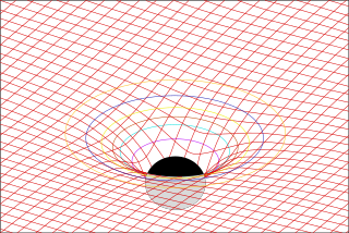
The stress–energy tensor, sometimes called the stress–energy–momentum tensor or the energy–momentum tensor, is a tensor physical quantity that describes the density and flux of energy and momentum in spacetime, generalizing the stress tensor of Newtonian physics. It is an attribute of matter, radiation, and non-gravitational force fields. This density and flux of energy and momentum are the sources of the gravitational field in the Einstein field equations of general relativity, just as mass density is the source of such a field in Newtonian gravity.

Linear elasticity is a mathematical model of how solid objects deform and become internally stressed due to prescribed loading conditions. It is a simplification of the more general nonlinear theory of elasticity and a branch of continuum mechanics.

The Richardson number (Ri) is named after Lewis Fry Richardson (1881–1953). It is the dimensionless number that expresses the ratio of the buoyancy term to the flow shear term:

<span class="mw-page-title-main">Onsager reciprocal relations</span> Relations between flows and forces, or gradients, in thermodynamic systems

In thermodynamics, the Onsager reciprocal relations express the equality of certain ratios between flows and forces in thermodynamic systems out of equilibrium, but where a notion of local equilibrium exists.

<span class="mw-page-title-main">Einstein–Hilbert action</span>

The Einstein–Hilbert action in general relativity is the action that yields the Einstein field equations through the stationary-action principle. With the (− + + +) metric signature, the gravitational part of the action is given as

<span class="mw-page-title-main">String vibration</span>

A vibration in a string is a wave. Resonance causes a vibrating string to produce a sound with constant frequency, i.e. constant pitch. If the length or tension of the string is correctly adjusted, the sound produced is a musical tone. Vibrating strings are the basis of string instruments such as guitars, cellos, and pianos.

The Hagen number (Hg) is a dimensionless number used in forced flow calculations. It is the forced flow equivalent of the Grashof number and was named after the German hydraulic engineer G. H. L. Hagen.

<span class="mw-page-title-main">Electromagnetic tensor</span> Mathematical object that describes the electromagnetic field in spacetime

In electromagnetism, the electromagnetic tensor or electromagnetic field tensor is a mathematical object that describes the electromagnetic field in spacetime. The field tensor was first used after the four-dimensional tensor formulation of special relativity was introduced by Hermann Minkowski. The tensor allows related physical laws to be written very concisely, and allows for the quantization of the electromagnetic field by Lagrangian formulation described below.

<span class="mw-page-title-main">Electromagnetic stress–energy tensor</span>

In relativistic physics, the electromagnetic stress–energy tensor is the contribution to the stress–energy tensor due to the electromagnetic field. The stress–energy tensor describes the flow of energy and momentum in spacetime. The electromagnetic stress–energy tensor contains the negative of the classical Maxwell stress tensor that governs the electromagnetic interactions.

<span class="mw-page-title-main">Covariant formulation of classical electromagnetism</span>

The covariant formulation of classical electromagnetism refers to ways of writing the laws of classical electromagnetism in a form that is manifestly invariant under Lorentz transformations, in the formalism of special relativity using rectilinear inertial coordinate systems. These expressions both make it simple to prove that the laws of classical electromagnetism take the same form in any inertial coordinate system, and also provide a way to translate the fields and forces from one frame to another. However, this is not as general as Maxwell's equations in curved spacetime or non-rectilinear coordinate systems.

<span class="mw-page-title-main">Maxwell's equations in curved spacetime</span> Electromagnetism in general relativity

In physics, Maxwell's equations in curved spacetime govern the dynamics of the electromagnetic field in curved spacetime or where one uses an arbitrary coordinate system. These equations can be viewed as a generalization of the vacuum Maxwell's equations which are normally formulated in the local coordinates of flat spacetime. But because general relativity dictates that the presence of electromagnetic fields induce curvature in spacetime, Maxwell's equations in flat spacetime should be viewed as a convenient approximation.

In the theory of general relativity, a stress–energy–momentum pseudotensor, such as the Landau–Lifshitz pseudotensor, is an extension of the non-gravitational stress–energy tensor that incorporates the energy–momentum of gravity. It allows the energy–momentum of a system of gravitating matter to be defined. In particular it allows the total of matter plus the gravitating energy–momentum to form a conserved current within the framework of general relativity, so that the total energy–momentum crossing the hypersurface of any compact space–time hypervolume vanishes.

<span class="mw-page-title-main">Newman–Penrose formalism</span> Notation in general relativity

The Newman–Penrose (NP) formalism is a set of notation developed by Ezra T. Newman and Roger Penrose for general relativity (GR). Their notation is an effort to treat general relativity in terms of spinor notation, which introduces complex forms of the usual variables used in GR. The NP formalism is itself a special case of the tetrad formalism, where the tensors of the theory are projected onto a complete vector basis at each point in spacetime. Usually this vector basis is chosen to reflect some symmetry of the spacetime, leading to simplified expressions for physical observables. In the case of the NP formalism, the vector basis chosen is a null tetrad: a set of four null vectors—two real, and a complex-conjugate pair. The two real members often asymptotically point radially inward and radially outward, and the formalism is well adapted to treatment of the propagation of radiation in curved spacetime. The Weyl scalars, derived from the Weyl tensor, are often used. In particular, it can be shown that one of these scalars— in the appropriate frame—encodes the outgoing gravitational radiation of an asymptotically flat system.

<span class="mw-page-title-main">Mathematical descriptions of the electromagnetic field</span> Formulations of electromagnetism

There are various mathematical descriptions of the electromagnetic field that are used in the study of electromagnetism, one of the four fundamental interactions of nature. In this article, several approaches are discussed, although the equations are in terms of electric and magnetic fields, potentials, and charges with currents, generally speaking.

In nonideal fluid dynamics, the Hagen–Poiseuille equation, also known as the Hagen–Poiseuille law, Poiseuille law or Poiseuille equation, is a physical law that gives the pressure drop in an incompressible and Newtonian fluid in laminar flow flowing through a long cylindrical pipe of constant cross section. It can be successfully applied to air flow in lung alveoli, or the flow through a drinking straw or through a hypodermic needle. It was experimentally derived independently by Jean Léonard Marie Poiseuille in 1838 and Gotthilf Heinrich Ludwig Hagen, and published by Poiseuille in 1840–41 and 1846. The theoretical justification of the Poiseuille law was given by George Stokes in 1845.

In fluid mechanics, dynamic similarity is the phenomenon that when there are two geometrically similar vessels with the same boundary conditions and the same Reynolds and Womersley numbers, then the fluid flows will be identical. This can be seen from inspection of the underlying Navier-Stokes equation, with geometrically similar bodies, equal Reynolds and Womersley Numbers the functions of velocity (u’,v’,w’) and pressure (P’) for any variation of flow.

<span class="mw-page-title-main">Falkner–Skan boundary layer</span> Boundary Layer

In fluid dynamics, the Falkner–Skan boundary layer describes the steady two-dimensional laminar boundary layer that forms on a wedge, i.e. flows in which the plate is not parallel to the flow. It is also representative of flow on a flat plate with an imposed pressure gradient along the plate length, a situation often encountered in wind tunnel flow. It is a generalization of the flat plate Blasius boundary layer in which the pressure gradient along the plate is zero.

Lagrangian field theory is a formalism in classical field theory. It is the field-theoretic analogue of Lagrangian mechanics. Lagrangian mechanics is used to analyze the motion of a system of discrete particles each with a finite number of degrees of freedom. Lagrangian field theory applies to continua and fields, which have an infinite number of degrees of freedom.

References

  1. Sander, C.J.; Holman, J.P. (1972). "Franz Grashof and the Grashof Number". Int. J. Heat Mass Transfer. 15 (3): 562–563. doi:10.1016/0017-9310(72)90220-7.
  2. 1 2 3 Incropera, Frank (2007). Fundamentals of Heat and Mass Transfer (6th ed.). Hoboken, NJ: Wiley. pp.  408, 599, 629. ISBN   9780471457282. OCLC   288958608.
  3. 1 2 Bird, R. Byron; Stewart, Warren E.; Lightfoot, Edwin N. (2002). Transport Phenomena (2nd ed.). New York: J. Wiley. pp.  318, 359. ISBN   9780471410775. OCLC   471520548.
  4. Shah, Nehad Ali; Animasaun, I.L.; Ibraheem, R.O.; Babatunde, H.A.; Sandeep, N.; Pop, I. (2018). "Scrutinization of the effects of Grashof number on the flow of different fluids driven by convection over various surfaces". Journal of Molecular Liquids. 249: 980–990. doi:10.1016/j.molliq.2017.11.042. ISSN   0167-7322.

Further reading