Scene rendered with RRV (simple implementation of radiosity renderer based on OpenGL) 79th iterationThe Cornell box, rendered with and without radiosity by BMRT
In 3D computer graphics, radiosity is an application of the finite element method to solving the rendering equation for scenes with surfaces that reflect light diffusely. Unlike rendering methods that use Monte Carlo algorithms (such as path tracing), which handle all types of light paths, typical radiosity only account for paths (represented by the code "LD*E") which leave a light source and are reflected diffusely some number of times (possibly zero) before hitting the eye. Radiosity is a global illuminationalgorithm in the sense that the illumination arriving on a surface comes not just directly from the light sources, but also from other surfaces reflecting light. Radiosity is viewpoint independent, which increases the calculations involved, but makes them useful for all viewpoints.
Radiosity methods were first developed in about 1950 in the engineering field of heat transfer. They were later refined specifically for the problem of rendering computer graphics in 1984–1985 by researchers at Cornell University[2] and Hiroshima University.[3]
Difference between standard direct illumination without shadow penumbra, and radiosity with shadow penumbra
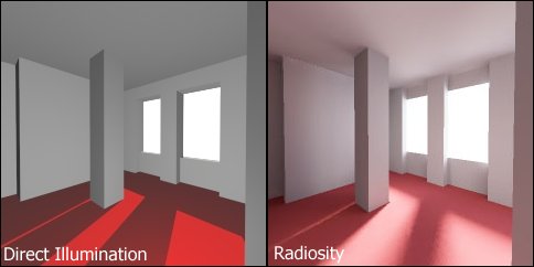
The inclusion of radiosity calculations in the rendering process often lends an added element of realism to the finished scene, because of the way it mimics real-world phenomena. Consider a simple room scene.
The image on the left was rendered with a typical direct illumination renderer. There are three types of lighting in this scene which have been specifically chosen and placed by the artist in an attempt to create realistic lighting: spot lighting with shadows (placed outside the window to create the light shining on the floor), ambient lighting (without which any part of the room not lit directly by a light source would be totally dark), and omnidirectional lighting without shadows (to reduce the flatness of the ambient lighting).
The image on the right was rendered using a radiosity algorithm. There is only one source of light: an image of the sky placed outside the window. The difference is marked. The room glows with light. Soft shadows are visible on the floor, and subtle lighting effects are noticeable around the room. Furthermore, the red color from the carpet has bled onto the grey walls, giving them a slightly warm appearance. None of these effects were specifically chosen or designed by the artist.
Overview of the radiosity algorithm
The surfaces of the scene to be rendered are each divided up into one or more smaller surfaces (patches). A view factor (also known as form factor) is computed for each pair of patches; it is a coefficient describing how well the patches can see each other. Patches that are far away from each other, or oriented at oblique angles relative to one another, will have smaller view factors. If other patches are in the way, the view factor will be reduced or zero, depending on whether the occlusion is partial or total.
The view factors are used as coefficients in a linear system of rendering equations. Solving this system yields the radiosity, or brightness, of each patch, taking into account diffuse interreflections and soft shadows.
Progressive radiosity solves the system iteratively with intermediate radiosity values for the patch, corresponding to bounce levels. That is, after each iteration, we know how the scene looks after one light bounce, after two passes, two bounces, and so forth. This is useful for getting an interactive preview of the scene. Also, the user can stop the iterations once the image looks good enough, rather than wait for the computation to numerically converge.
As the algorithm iterates, light can be seen to flow into the scene, as multiple bounces are computed. Individual patches are visible as squares on the walls and floor.
Another common method for solving the radiosity equation is "shooting radiosity," which iteratively solves the radiosity equation by "shooting" light from the patch with the most energy at each step. After the first pass, only those patches which are in direct line of sight of a light-emitting patch will be illuminated. After the second pass, more patches will become illuminated as the light begins to bounce around the scene. The scene continues to grow brighter and eventually reaches a steady state.
Mathematical formulation
The basic radiosity method has its basis in the theory of thermal radiation, since radiosity relies on computing the amount of light energy transferred among surfaces. In order to simplify computations, the method assumes that all scattering is perfectly diffuse. Surfaces are typically discretized into quadrilateral or triangular elements over which a piecewise polynomial function is defined.
After this breakdown, the amount of light energy transfer can be computed by using the known reflectivity of the reflecting patch, combined with the view factor of the two patches. This dimensionless quantity is computed from the geometric orientation of two patches, and can be thought of as the fraction of the total possible emitting area of the first patch which is covered by the second.
More correctly, radiosity B is the energy per unit area leaving the patch surface per discrete time interval and is the combination of emitted and reflected energy:
where:
B(x)i dAi is the total energy leaving a small area dAi around a point x.
E(x)i dAi is the emitted energy.
ρ(x) is the reflectivity of the point, giving reflected energy per unit area by multiplying by the incident energy per unit area (the total energy which arrives from other patches).
S denotes that the integration variable x' runs over all the surfaces in the scene
r is the distance between x and x'
θx and θx' are the angles between the line joining x and x' and vectors normal to the surface at x and x' respectively.
Vis(x,x' ) is a visibility function, defined to be 1 if the two points x and x' are visible from each other, and 0 if they are not.
The geometrical form factor (or "projected solid angle") Fij.
Fij can be obtained by projecting the element Aj onto the surface of a unit hemisphere, and then projecting that in turn onto a unit circle around the point of interest in the plane of Ai. The form factor is then equal to the proportion of the unit circle covered by this projection.
Form factors obey the reciprocity relation AiFij = AjFji
If the surfaces are approximated by a finite number of planar patches, each of which is taken to have a constant radiosity Bi and reflectivity ρi, the above equation gives the discrete radiosity equation,
where Fij is the geometrical view factor for the radiation leaving j and hitting patch i.
This equation can then be applied to each patch. The equation is monochromatic, so color radiosity rendering requires calculation for each of the required colors.
Solution methods
The equation can formally be solved as matrix equation, to give the vector solution:
This gives the full "infinite bounce" solution for B directly. However the number of calculations to compute the matrix solution scales according to n3, where n is the number of patches. This becomes prohibitive for realistically large values of n.
Instead, the equation can more readily be solved iteratively, by repeatedly applying the single-bounce update formula above. Formally, this is a solution of the matrix equation by Jacobi iteration. Because the reflectivities ρi are less than 1, this scheme converges quickly, typically requiring only a handful of iterations to produce a reasonable solution. Other standard iterative methods for matrix equation solutions can also be used, for example the Gauss–Seidel method, where updated values for each patch are used in the calculation as soon as they are computed, rather than all being updated synchronously at the end of each sweep. The solution can also be tweaked to iterate over each of the sending elements in turn in its main outermost loop for each update, rather than each of the receiving patches. This is known as the shooting variant of the algorithm, as opposed to the gathering variant. Using the view factor reciprocity, AiFij = AjFji, the update equation can also be re-written in terms of the view factor Fji seen by each sending patch Aj:
This is sometimes known as the "power" formulation, since it is now the total transmitted power of each element that is being updated, rather than its radiosity.
The view factorFij itself can be calculated in a number of ways. Early methods used a hemicube (an imaginary cube centered upon the first surface to which the second surface was projected, devised by Michael F. Cohen and Donald P. Greenberg in 1985). The surface of the hemicube was divided into pixel-like squares, for each of which a view factor can be readily calculated analytically. The full form factor could then be approximated by adding up the contribution from each of the pixel-like squares. The projection onto the hemicube, which could be adapted from standard methods for determining the visibility of polygons, also solved the problem of intervening patches partially obscuring those behind.
However all this was quite computationally expensive, because ideally form factors must be derived for every possible pair of patches, leading to a quadratic increase in computation as the number of patches increased. This can be reduced somewhat by using a binary space partitioning tree to reduce the amount of time spent determining which patches are completely hidden from others in complex scenes; but even so, the time spent to determine the form factor still typically scales as n log n. New methods include adaptive integration.[4]
Sampling approaches
The form factors Fij themselves are not in fact explicitly needed in either of the update equations; neither to estimate the total intensity ΣjFijBj gathered from the whole view, nor to estimate how the power AjBj being radiated is distributed. Instead, these updates can be estimated by sampling methods, without ever having to calculate form factors explicitly. Since the mid 1990s such sampling approaches have been the methods most predominantly used for practical radiosity calculations.
The gathered intensity can be estimated by generating a set of samples in the unit circle, lifting these onto the hemisphere, and then seeing what was the radiosity of the element that a ray incoming in that direction would have originated on. The estimate for the total gathered intensity is then just the average of the radiosities discovered by each ray. Similarly, in the power formulation, power can be distributed by generating a set of rays from the radiating element in the same way, and spreading the power to be distributed equally between each element a ray hits.
This is essentially the same distribution that a path-tracing program would sample in tracing back one diffuse reflection step; or that a bidirectional ray-tracing program would sample to achieve one forward diffuse reflection step when light source mapping forwards. The sampling approach therefore to some extent represents a convergence between the two techniques, the key difference remaining that the radiosity technique aims to build up a sufficiently accurate map of the radiance of all the surfaces in the scene, rather than just a representation of the current view.
A modern render of the Utah teapot. Radiosity was used for all diffuse illumination in this scene.
Limitations
Typical radiosity methods only account for light paths of the form LD*E, i.e. paths which start at a light source and make multiple diffuse bounces before reaching the eye. Although there are several approaches to integrating other illumination effects such as specular[5] and glossy[6] reflections, radiosity-based methods are generally not used to solve the complete rendering equation.
Basic radiosity also has trouble resolving sudden changes in visibility (e.g. hard-edged shadows) because coarse, regular discretization into piecewise constant elements corresponds to a low-pass box filter of the spatial domain. Discontinuity meshing uses knowledge of visibility events to generate a more intelligent discretization.
Confusion about terminology
Radiosity was perhaps the first rendering algorithm in widespread use which accounted for diffuse indirect lighting. Earlier rendering algorithms, such as Whitted-styleray tracing were capable of computing effects such as reflections, refractions, and shadows, but despite being highly global phenomena, these effects were not commonly referred to as "global illumination." As a consequence, the terms "diffuse interreflection" and "radiosity" both became confused with "global illumination" in popular parlance. However, the three are distinct concepts.
The radiosity method, in the context of computer graphics, derives from (and is fundamentally the same as) the radiosity method in heat transfer. In this context, radiosity is the total radiative flux (both reflected and re-radiated) leaving a surface; this is also sometimes known as radiant exitance. Calculation of radiosity, rather than surface temperatures, is a key aspect of the radiosity method that permits linear matrix methods to be applied to the problem.
↑Wallace, John R.; Cohen, Michael F.; Greenberg, Donald P. (August 1987). "A two-pass solution to the rendering equation: A synthesis of ray tracing and radiosity methods". ACM SIGGRAPH Computer Graphics. 21 (4): 311–320. doi:10.1145/37402.37438. ISSN0097-8930.
RADical, by Parag Chaudhuri (an implementation of shooting & sorting variant of progressive radiosity algorithm with OpenGL acceleration, extending from GLUTRAD by Colbeck)
This page is based on this Wikipedia article Text is available under the CC BY-SA 4.0 license; additional terms may apply. Images, videos and audio are available under their respective licenses.