Uniform distribution (continuous)

Last updated
Uniform
Probability density function
Uniform Distribution PDF SVG.svg
Using maximum convention
Cumulative distribution function
Uniform cdf.svg
Notation or
Parameters
Support
PDF
CDF
Mean
Median
Mode any value in
Variance
Skewness 0
Ex. kurtosis
Entropy
MGF
CF

In probability theory and statistics, the continuous uniform distribution or rectangular distribution is a family of symmetric probability distributions. The distribution describes an experiment where there is an arbitrary outcome that lies between certain bounds. [1] The bounds are defined by the parameters, a and b, which are the minimum and maximum values. The interval can be either be closed (eg. [a, b]) or open (eg. (a, b)). [2] Therefore, the distribution is often abbreviated U (a, b), where U stands for uniform distribution. [1] The difference between the bounds defines the interval length; all intervals of the same length on the distribution's support are equally probable. It is the maximum entropy probability distribution for a random variable X under no constraint other than that it is contained in the distribution's support. [3]

Contents

Definitions

Probability density function

The probability density function of the continuous uniform distribution is:

The values of f(x) at the two boundaries a and b are usually unimportant because they do not alter the values of the integrals of f(x) dx over any interval, nor of x f(x) dx or any higher moment. Sometimes they are chosen to be zero, and sometimes chosen to be 1/(b  a). The latter is appropriate in the context of estimation by the method of maximum likelihood. In the context of Fourier analysis, one may take the value of f(a) or f(b) to be 1/(2(b  a)), since then the inverse transform of many integral transforms of this uniform function will yield back the function itself, rather than a function which is equal "almost everywhere", i.e. except on a set of points with zero measure. Also, it is consistent with the sign function which has no such ambiguity.

Graphically, the probability density function is portrayed as a rectangle where (b-a) is the base and (1/(b-a)) is the height. As the distance between a and b increases, the density at any particular value within the distribution boundaries decreases. [4] Since the probability density function integrates to 1, the height of the probability density function decreases as the base length increases. [4]

In terms of mean μ and variance σ2, the probability density may be written as:

Example 1. Using the Uniform Probability Density Function [5]

For random variable X

X~U(0,23)

Find P(2 < X < 18):

P(2 < X < 18) = (18-2)*(1/(23-0)) = 16/23.

In graphical representation of uniform distribution function [f(x) vs x], the area under the curve within the specified bounds displays the probability (shaded area is depicted as a rectangle). For this specific example above, the base would be (18-2) and the height would be (1/23). [5]

Example 2. Using the Uniform Probability Density Function (Conditional) [5]

For random variable X

X~U(0,23)

Find P(12 < X | X > 8):

P(X > 12 | X > 8) = (23-12)*(1/(23-8))=11/15.

The example above is for a conditional probability case for the uniform distribution: given X > 8 is true, what is the probability that X > 12. Conditional probability changes the sample space so a new interval length (b-a) has to be calculated, where b is 23 and a is 8. [5] The graphical representation would still follow Example 1, where the area under the curve within the specified bounds displays the probability and the base of the rectangle would be (23-12) and the height (1/15). [5]

Cumulative distribution function

The cumulative distribution function is:

Its inverse is:

In mean and variance notation, the cumulative distribution function is:

and the inverse is:

Generating functions

Moment-generating function

The moment-generating function is: [6]

[7]

from which we may calculate the raw moments mk

For the special case a = b, that is, for

the moment-generating functions reduces to the simple form

For a random variable following this distribution, the expected value is then m1 = (a + b)/2 and the variance is m2  m12 = (b  a)2/12.

Cumulant-generating function

For n  2, the nth cumulant of the uniform distribution on the interval [-1/2, 1/2] is Bn/n, where Bn is the nth Bernoulli number. [8]

Standard uniform

Restricting and , the resulting distribution U(0,1) is called a standard uniform distribution.

One interesting property of the standard uniform distribution is that if u1 has a standard uniform distribution, then so does 1-u1. This property can be used for generating antithetic variates, among other things. In other words, this property is known as the inversion method where the continuous standard uniform distribution can be used to generate random numbers for any other continuous distribution. [4] If u is a uniform random number with standard uniform distribution (0,1), then generates a random number x from any continuous distribution with the specified cumulative distribution function F. [4]

Relationship to other functions

As long as the same conventions are followed at the transition points, the probability density function may also be expressed in terms of the Heaviside step function:

or in terms of the rectangle function

There is no ambiguity at the transition point of the sign function. Using the half-maximum convention at the transition points, the uniform distribution may be expressed in terms of the sign function as:

Properties

Moments

The mean (first moment) of the distribution is:

The second moment of the distribution is:

In general, the n-th moment of the uniform distribution is:

The variance (second central moment) is:

Order statistics

Let X1, ..., Xn be an i.i.d. sample from U(0,1). Let X(k) be the kth order statistic from this sample. Then the probability distribution of X(k) is a Beta distribution with parameters k and nk + 1. The expected value is

This fact is useful when making Q–Q plots.

The variances are

See also: Order statistic § Probability distributions of order statistics

Uniformity

The probability that a uniformly distributed random variable falls within any interval of fixed length is independent of the location of the interval itself (but it is dependent on the interval size), so long as the interval is contained in the distribution's support.

To see this, if X ~ U(a,b) and [x, x+d] is a subinterval of [a,b] with fixed d> 0, then

which is independent of x. This fact motivates the distribution's name.

Generalization to Borel sets

This distribution can be generalized to more complicated sets than intervals. If S is a Borel set of positive, finite measure, the uniform probability distribution on S can be specified by defining the pdf to be zero outside S and constantly equal to 1/K on S, where K is the Lebesgue measure of S.

Statistical inference

Estimation of parameters

Estimation of maximum

Minimum-variance unbiased estimator

Given a uniform distribution on [0, b] with unknown b, the minimum-variance unbiased estimator (UMVUE) for the maximum is given by

where m is the sample maximum and k is the sample size, sampling without replacement (though this distinction almost surely makes no difference for a continuous distribution). This follows for the same reasons as estimation for the discrete distribution, and can be seen as a very simple case of maximum spacing estimation. This problem is commonly known as the German tank problem, due to application of maximum estimation to estimates of German tank production during World War II.

Maximum likelihood estimator

The maximum likelihood estimator is given by:

where m is the sample maximum, also denoted as the maximum order statistic of the sample.

Method of moment estimator

The method of moments estimator is given by:

where is the sample mean.

Estimation of midpoint

The midpoint of the distribution (a + b) / 2 is both the mean and the median of the uniform distribution. Although both the sample mean and the sample median are unbiased estimators of the midpoint, neither is as efficient as the sample mid-range, i.e. the arithmetic mean of the sample maximum and the sample minimum, which is the UMVU estimator of the midpoint (and also the maximum likelihood estimate).

Confidence interval

For the maximum

Let X1, X2, X3, ..., Xn be a sample from U( 0, L ) where L is the population maximum. Then X(n) = max( X1, X2, X3, ..., Xn ) has the density [9]

The confidence interval for the estimated population maximum is then ( X(n), X(n) / α1/n ) where 100(1  α)% is the confidence level sought. In symbols

Hypothesis testing

In statistics, when a p-value is used as a test statistic for a simple null hypothesis, and the distribution of the test statistic is continuous, then the p-value is uniformly distributed between 0 and 1 if the null hypothesis is true.

Occurrence and applications

The probabilities for uniform distribution function are simple to calculate due to the simplicity of the function form. [2] Therefore, there are various applications that this distribution can be used for as shown below: hypothesis testing situations, random sampling cases, finance, etc. Furthermore, generally, experiments of physical origin follow a uniform distribution (eg. emission of radioactive particles). [1] However, it is important to note that in any application, there is the unchanging assumption that the probability of falling in an interval of fixed length is constant. [2]

Economics example for uniform distribution

In the field of economics, usually demand and replenishment may not follow the expected normal distribution. As a result, other distribution models are used to better predict probabilities and trends such as Bernoulli process. [10] But according to Wanke (2008), in the particular case of investigating lead-time for inventory management at the beginning of the life cycle when a completely new product is being analyzed, the uniform distribution proves to be more useful. [10] In this situation, other distribution may not be viable since there is no existing data on the new product or that the demand history is unavailable so there isn't really an appropriate or known distribution. [10] The uniform distribution would be ideal in this situation since the random variable of lead-time (related to demand) is unknown for the new product but the results are likely to range between a plausible range of two values. [10] The lead-time would thus represent the random variable. From the uniform distribution model, other factors related to lead-time were able to be calculated such as cycle service level and shortage per cycle. It was also noted that the uniform distribution was also used due to the simplicity of the calculations. [10]

Sampling from an arbitrary distribution

The uniform distribution is useful for sampling from arbitrary distributions. A general method is the inverse transform sampling method, which uses the cumulative distribution function (CDF) of the target random variable. This method is very useful in theoretical work. Since simulations using this method require inverting the CDF of the target variable, alternative methods have been devised for the cases where the cdf is not known in closed form. One such method is rejection sampling.

The normal distribution is an important example where the inverse transform method is not efficient. However, there is an exact method, the Box–Muller transformation, which uses the inverse transform to convert two independent uniform random variables into two independent normally distributed random variables.

Quantization error

In analog-to-digital conversion a quantization error occurs. This error is either due to rounding or truncation. When the original signal is much larger than one least significant bit (LSB), the quantization error is not significantly correlated with the signal, and has an approximately uniform distribution. The RMS error therefore follows from the variance of this distribution.

Computational methods

Sampling from a uniform distribution

There are many applications in which it is useful to run simulation experiments. Many programming languages come with implementations to generate pseudo-random numbers which are effectively distributed according to the standard uniform distribution.

If u is a value sampled from the standard uniform distribution, then the value a + (ba)u follows the uniform distribution parametrised by a and b, as described above.

History

While the historical origins in the conception of uniform distribution are inconclusive, it is speculated that the term 'uniform' arose from the concept of equiprobability in dice games (note that the dice games would have discrete and not continuous uniform sample space). Equiprobability was mentioned in Gerolamo Cardano's Liber de Ludo Aleae, a manual written in 16th century and detailed on advanced probability calculus in relation to dice. [11]

See also

Related Research Articles

Binomial distribution Probability distribution

In probability theory and statistics, the binomial distribution with parameters n and p is the discrete probability distribution of the number of successes in a sequence of n independent experiments, each asking a yes–no question, and each with its own boolean-valued outcome: success/yes/true/one or failure/no/false/zero. A single success/failure experiment is also called a Bernoulli trial or Bernoulli experiment and a sequence of outcomes is called a Bernoulli process; for a single trial, i.e., n = 1, the binomial distribution is a Bernoulli distribution. The binomial distribution is the basis for the popular binomial test of statistical significance.

Cumulative distribution function Probability that random variable X is less than or equal to x.

In probability theory and statistics, the cumulative distribution function (CDF) of a real-valued random variable , or just distribution function of , evaluated at , is the probability that will take a value less than or equal to .

Normal distribution Probability distribution

In probability theory, a normaldistribution is a type of continuous probability distribution for a real-valued random variable. The general form of its probability density function is

Random variable Variable representing a random phenomenon

In probability and statistics, a random variable, random quantity, aleatory variable, or stochastic variable is described informally as a variable whose values depend on outcomes of a random phenomenon. The formal mathematical treatment of random variables is a topic in probability theory. In that context, a random variable is understood as a measurable function defined on a probability space that maps from the sample space to the real numbers.

In probability theory, the central limit theorem (CLT) establishes that, in some situations, when independent random variables are added, their properly normalized sum tends toward a normal distribution even if the original variables themselves are not normally distributed. The theorem is a key concept in probability theory because it implies that probabilistic and statistical methods that work for normal distributions can be applicable to many problems involving other types of distributions.

Students <i>t</i>-distribution Probability distribution

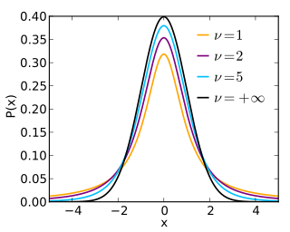
In probability and statistics, Student's t-distribution is any member of a family of continuous probability distributions that arises when estimating the mean of a normally distributed population in situations where the sample size is small and the population standard deviation is unknown. It was developed by William Sealy Gosset under the pseudonym Student.

In statistics, maximum likelihood estimation (MLE) is a method of estimating the parameters of a probability distribution by maximizing a likelihood function, so that under the assumed statistical model the observed data is most probable. The point in the parameter space that maximizes the likelihood function is called the maximum likelihood estimate. The logic of maximum likelihood is both intuitive and flexible, and as such the method has become a dominant means of statistical inference.

In probability theory, Chebyshev's inequality guarantees that, for a wide class of probability distributions, no more than a certain fraction of values can be more than a certain distance from the mean. Specifically, no more than 1/k2 of the distribution's values can be more than k standard deviations away from the mean. The rule is often called Chebyshev's theorem, about the range of standard deviations around the mean, in statistics. The inequality has great utility because it can be applied to any probability distribution in which the mean and variance are defined. For example, it can be used to prove the weak law of large numbers.

Order statistic kth smallest value in a statistical sample

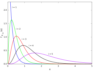
In statistics, the kth order statistic of a statistical sample is equal to its kth-smallest value. Together with rank statistics, order statistics are among the most fundamental tools in non-parametric statistics and inference.

Rayleigh distribution

In probability theory and statistics, the Rayleigh distribution is a continuous probability distribution for nonnegative-valued random variables. It is essentially a chi distribution with two degrees of freedom.

In statistics, a confidence interval (CI) is a type of estimate computed from the statistics of the observed data. This proposes a range of plausible values for an unknown parameter. The interval has an associated confidence level that the true parameter is in the proposed range. Given observations and a confidence level , a valid confidence interval has a probability of containing the true underlying parameter. The level of confidence can be chosen by the investigator. In general terms, a confidence interval for an unknown parameter is based on sampling the distribution of a corresponding estimator.

In statistical inference, specifically predictive inference, a prediction interval is an estimate of an interval in which a future observation will fall, with a certain probability, given what has already been observed. Prediction intervals are often used in regression analysis.

Triangular distribution Probability distribution

In probability theory and statistics, the triangular distribution is a continuous probability distribution with lower limit a, upper limit b and mode c, where a < b and a ≤ c ≤ b.

Lévy distribution continuous probability distribution for a non-negative random variable

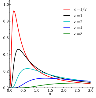
In probability theory and statistics, the Lévy distribution, named after Paul Lévy, is a continuous probability distribution for a non-negative random variable. In spectroscopy, this distribution, with frequency as the dependent variable, is known as a van der Waals profile. It is a special case of the inverse-gamma distribution. It is a stable distribution.

Truncated normal distribution probability distribution derived from that of a normally distributed random variable by bounding the random variable from below, above or both

In probability and statistics, the truncated normal distribution is the probability distribution derived from that of a normally distributed random variable by bounding the random variable from either below or above. The truncated normal distribution has wide applications in statistics and econometrics. For example, it is used to model the probabilities of the binary outcomes in the probit model and to model censored data in the Tobit model.

Half-normal distribution probability distribution

In probability theory and statistics, the half-normal distribution is a special case of the folded normal distribution.

Poisson distribution discrete probability distribution

In probability theory and statistics, the Poisson distribution, named after French mathematician Siméon Denis Poisson, is a discrete probability distribution that expresses the probability of a given number of events occurring in a fixed interval of time or space if these events occur with a known constant mean rate and independently of the time since the last event. The Poisson distribution can also be used for the number of events in other specified intervals such as distance, area or volume.

A product distribution is a probability distribution constructed as the distribution of the product of random variables having two other known distributions. Given two statistically independent random variables X and Y, the distribution of the random variable Z that is formed as the product

In statistics and probability theory, the nonparametric skew is a statistic occasionally used with random variables that take real values. It is a measure of the skewness of a random variable's distribution—that is, the distribution's tendency to "lean" to one side or the other of the mean. Its calculation does not require any knowledge of the form of the underlying distribution—hence the name nonparametric. It has some desirable properties: it is zero for any symmetric distribution; it is unaffected by a scale shift; and it reveals either left- or right-skewness equally well. In some statistical samples it has been shown to be less powerful than the usual measures of skewness in detecting departures of the population from normality.

In probability theory and statistics, an inverse distribution is the distribution of the reciprocal of a random variable. Inverse distributions arise in particular in the Bayesian context of prior distributions and posterior distributions for scale parameters. In the algebra of random variables, inverse distributions are special cases of the class of ratio distributions, in which the numerator random variable has a degenerate distribution.

References

  1. 1 2 3 Dekking, Michel (2005). A modern introduction to probability and statistics : understanding why and how . London, UK: Springer. pp.  60–61. ISBN   978-1-85233-896-1.
  2. 1 2 3 Walpole, Ronald; et al. (2012). Probability & Statistics for Engineers and Scientists. Boston, USA: Prentice Hall. pp. 171–172. ISBN   978-0-321-62911-1.
  3. Park, Sung Y.; Bera, Anil K. (2009). "Maximum entropy autoregressive conditional heteroskedasticity model". Journal of Econometrics . 150 (2): 219–230. CiteSeerX   10.1.1.511.9750 . doi:10.1016/j.jeconom.2008.12.014.
  4. 1 2 3 4 "Uniform Distribution (Continuous)". MathWorks. 2019. Retrieved November 22, 2019.
  5. 1 2 3 4 5 Illowsky, Barbara; et al. (2013). Introductory Statistics. Rice University, Houston, Texas, USA: OpenStax College. pp.  296–304. ISBN   978-1-938168-20-8.
  6. Casella & Berger 2001 , p. 626
  7. https://www.stat.washington.edu/~nehemyl/files/UW_MATH-STAT395_moment-functions.pdf
  8. https://galton.uchicago.edu/~wichura/Stat304/Handouts/L18.cumulants.pdf
  9. Nechval KN, Nechval NA, Vasermanis EK, Makeev VY (2002) Constructing shortest-length confidence intervals. Transport and Telecommunication 3 (1) 95-103
  10. 1 2 3 4 5 Wanke, Peter (2008). "The uniform distribution as a first practical approach to new product inventory management". International Journal of Production Economics. 114 (2): 811–819. doi:10.1016/j.ijpe.2008.04.004 via Research Gate.
  11. Bellhouse, David (May 2005). "Decoding Cardano's Liber de Ludo". Historia Mathematica. 32: 180–202. doi: 10.1016/j.hm.2004.04.001 .

Further reading