Flight dynamics (spacecraft)

This article is about flight dynamics of spacecraft. For aircraft flight dynamics, see Flight dynamics (aircraft). For attitude control of spacecraft, see Attitude control.

Flight path of the Apollo 11 human lunar landing mission, July 1969

Spacecraft flight dynamics is the application of mechanical dynamics to model how the external forces acting on a space vehicle or spacecraft determine its flight path. These forces are primarily of three types: propulsive force provided by the vehicle's engines; gravitational force exerted by the Earth and other celestial bodies; and aerodynamic lift and drag (when flying in the atmosphere of the Earth or other body, such as Mars or Venus).

The principles of flight dynamics are used to model a vehicle's powered flight during launch from the Earth; a spacecraft's orbital flight; maneuvers to change orbit; translunar and interplanetary flight; launch from and landing on a celestial body, with or without an atmosphere; entry through the atmosphere of the Earth or other celestial body; and attitude control. They are generally programmed into a vehicle's inertial navigation systems, and monitored on the ground by a member of the flight controller team known in NASA as the flight dynamics officer, or in the European Space Agency as the spacecraft navigator.

Flight dynamics depends on the disciplines of propulsion, aerodynamics, and astrodynamics (orbital mechanics and celestial mechanics). It cannot be reduced to simply attitude control; real spacecraft do not have steering wheels or tillers like airplanes or ships. Unlike the way fictional spaceships are portrayed, a spacecraft actually does not bank to turn in outer space, where its flight path depends strictly on the gravitational forces acting on it and the propulsive maneuvers applied.

Basic principles

A space vehicle's flight is determined by application of Newton's second law of motion:

${\displaystyle \mathbf {F} =m\mathbf {a} ,}$

where F is the vector sum of all forces exerted on the vehicle, m is its current mass, and a is the acceleration vector, the instantaneous rate of change of velocity (v), which in turn is the instantaneous rate of change of displacement. Solving for a, acceleration equals the force sum divided by mass. Acceleration is integrated over time to get velocity, and velocity is in turn integrated to get position.

Flight dynamics calculations are handled by computerized guidance systems aboard the vehicle; the status of the flight dynamics is monitored on the ground during powered maneuvers by a member of the flight controller team known in NASA's Human Spaceflight Center as the flight dynamics officer, or in the European Space Agency as the spacecraft navigator. ^[1]

For powered atmospheric flight, the three main forces which act on a vehicle are propulsive force, aerodynamic force, and gravitation. Other external forces such as centrifugal force, Coriolis force, and solar radiation pressure are generally insignificant due to the relatively short time of powered flight and small size of spacecraft, and may generally be neglected in simplified performance calculations. ^[2]

Propulsion

The thrust of a rocket engine, in the general case of operation in an atmosphere, is approximated by: ^[3]

${\displaystyle F={\dot {m}}\;v_{e}={\dot {m}}\;v_{e-opt}+A_{e}(p_{e}-p_{amb})}$

where:
${\displaystyle {\dot {m}}}$	=  exhaust gas mass flow
${\displaystyle v_{e}}$	=  effective exhaust velocity (sometimes otherwise denoted as c in publications)
${\displaystyle v_{e-opt}}$	=  effective jet velocity when Pamb = Pe
${\displaystyle A_{e}}$	=  flow area at nozzle exit plane (or the plane where the jet leaves the nozzle if separated flow)
${\displaystyle p_{e}}$	=  static pressure at nozzle exit plane
${\displaystyle p_{amb}}$	=  ambient (or atmospheric) pressure

The effective exhaust velocity of the rocket propellant is proportional to the vacuum specific impulse and affected by the atmospheric pressure: ^[4]

${\displaystyle {v_{e}}=(I_{sp-vac}-(A_{e}\,p_{amb})/{\dot {m}})\cdot g_{0}}$

where:

${\displaystyle I_{sp-vac}}$ has units of seconds

${\displaystyle g_{0}}$ is the gravitational acceleration at the surface of the Earth

The specific impulse relates the delta-v capacity to the quantity of propellant consumed according to the Tsiolkovsky rocket equation: ^[5]

${\displaystyle \Delta v\ =v_{e}\ln {\frac {m_{0}}{m_{1}}}}$

where:

${\displaystyle m_{0}}$ is the initial total mass, including propellant, in kg (or lb)

${\displaystyle m_{1}}$ is the final total mass in kg (or lb)

${\displaystyle v_{e}}$ is the effective exhaust velocity in m/s (or ft/s)

${\displaystyle \Delta v\ }$ is the delta-v in m/s (or ft/s)

Aerodynamic force

Aerodynamic forces, present near a body with significant atmosphere such as Earth, Mars or Venus, are analyzed as: lift, defined as the force component perpendicular to the direction of flight (not necessarily upward to balance gravity, as for an airplane); and drag, the component parallel to, and in the opposite direction of flight. Lift and drag are modeled as the products of a coefficient times dynamic pressure acting on a reference area: ^[6]

${\displaystyle \mathbf {L} =C_{L}qA_{\text{ref}}}$

${\displaystyle \mathbf {D} =C_{D}qA_{\text{ref}}}$

where:

• C_L is roughly linear with α, the angle of attack between the vehicle axis and the direction of flight (up to a limiting value), and is 0 at α = 0 for an axisymmetric body;
• C_D varies with α²;
• C_L and C_D vary with Reynolds number and Mach number;
• q, the dynamic pressure, is equal to 1/2 ρv², where ρ is atmospheric density, modeled for Earth as a function of altitude in the International Standard Atmosphere (using an assumed temperature distribution, hydrostatic pressure variation, and the ideal gas law); and
• A_ref is a characteristic area of the vehicle, such as cross-sectional area at the maximum diameter.

Gravitation

The gravitational force that a celestial body exerts on a space vehicle is modeled with the body and vehicle taken as point masses; the bodies (Earth, Moon, etc.) are simplified as spheres; and the mass of the vehicle is much smaller than the mass of the body so that its effect on the gravitational acceleration can be neglected. Therefore the gravitational force is calculated by:

${\displaystyle \mathbf {W} =m\cdot g}$

where:

${\displaystyle W}$ is the gravitational force (weight);

${\displaystyle m}$ is the space vehicle's mass; and

${\displaystyle r}$ is the radial distance of the vehicle to the planet's center; and

${\displaystyle r_{0}}$ is the radial distance from the planet's surface to its center; and

${\displaystyle g_{0}}$ is the gravitational acceleration at the surface of the planet

g is the gravitational acceleration at altitude, which varies with the inverse square of the radial distance to the planet's center:

${\displaystyle g=g_{0}\left({\frac {r_{0}}{r}}\right)^{2}\,}$ ^[7]

Powered flight

The equations of motion used to describe powered flight of a vehicle during launch can be as complex as six degrees of freedom for in-flight calculations, or as simple as two degrees of freedom for preliminary performance estimates. In-flight calculations will take perturbation factors into account such as the Earth's oblateness and non-uniform mass distribution; and gravitational forces of all nearby bodies, including the Moon, Sun, and other planets. Preliminary estimates can make some simplifying assumptions: a spherical, uniform planet; the vehicle can be represented as a point mass; solution of the flight path presents a two-body problem; and the local flight path lies in a single plane) with reasonably small loss of accuracy. ^[7]

Velocity, position, and force vectors acting on a space vehicle during launch

The general case of a launch from Earth must take engine thrust, aerodynamic forces, and gravity into account. The acceleration equation can be reduced from vector to scalar form by resolving it into its tangential (speed ${\displaystyle v}$) and angular (flight path angle ${\displaystyle \theta }$ relative to local vertical) time rate-of-change components relative to the launch pad. The two equations thus become:

${\displaystyle {\dot {v}}={\frac {F\cos \alpha }{m}}-{\frac {D}{m}}-g\cos \theta \,}$

${\displaystyle {\dot {\theta }}={\frac {F\sin \alpha }{mv}}+{\frac {L}{mv}}+\left({\frac {g}{v}}-{\frac {v}{r}}\right)\sin \theta ,\,}$

where:

F is the engine thrust;

α is the angle of attack;

m is the vehicle's mass;

D is the vehicle's aerodynamic drag;

L is its aerodynamic lift;

r is the radial distance to the planet's center; and

g is the gravitational acceleration at altitude.

Mass decreases as propellant is consumed and rocket stages, engines or tanks are shed (if applicable).

The planet-fixed values of v and θ at any time in the flight are then determined by numerical integration of the two rate equations from time zero (when both v and θ are 0):

${\displaystyle v=\int _{t_{0}}^{t}{\dot {v}}\,dt}$

${\displaystyle \theta =\int _{t_{0}}^{t}{\dot {\theta }}\,dt}$

Finite element analysis can be used to integrate the equations, by breaking the flight into small time increments.

For most launch vehicles, relatively small levels of lift are generated, and a gravity turn is employed, depending mostly on the third term of the angle rate equation. At the moment of liftoff, when angle and velocity are both zero, the theta-dot equation is mathematically indeterminate and cannot be evaluated until velocity becomes non-zero shortly after liftoff. But notice at this condition, the only force which can cause the vehicle to pitch over is the engine thrust acting at a non-zero angle of attack (first term) and perhaps a slight amount of lift (second term), until a non-zero pitch angle is attained. In the gravity turn, pitch-over is initiated by applying an increasing angle of attack (by means of gimbaled engine thrust), followed by a gradual decrease in angle of attack through the remainder of the flight. ^{[7] [8]}

Once velocity and flight path angle are known, altitude ${\displaystyle h}$ and downrange distance ${\displaystyle s}$ are computed as: ^[7]

Velocity and force vectors acting on a space vehicle during powered descent and landing

${\displaystyle h=\int _{t_{0}}^{t}v\cos \theta \,dt}$

${\displaystyle r=r_{0}+h\,}$

${\displaystyle s=r_{0}\int _{t_{0}}^{t}{\frac {v}{r}}\sin \theta \,dt}$

The planet-fixed values of v and θ are converted to space-fixed (inertial) values with the following conversions: ^[7]

${\displaystyle v_{s}={\sqrt {v^{2}+2\omega rv\cos \varphi \sin \theta \sin A_{z}+(\omega r\cos \theta )^{2}}},}$

where ω is the planet's rotational rate in radians per second, φ is the launch site latitude, and A_z is the launch azimuth angle.

${\displaystyle \theta _{s}=\arccos \left({\frac {v\cos \theta }{v_{s}}}\right)}$

Final v_s, θ_s and r must match the requirements of the target orbit as determined by orbital mechanics (see Orbital flight, above), where final v_s is usually the required periapsis (or circular) velocity, and final θ_s is 90 degrees. A powered descent analysis would use the same procedure, with reverse boundary conditions.

Orbital flight

Further information: Orbital mechanics

Orbital mechanics are used to calculate flight in orbit about a central body. For sufficiently high orbits (generally at least 190 kilometers (100 nautical miles) in the case of Earth), aerodynamic force may be assumed to be negligible for relatively short term missions (though a small amount of drag may be present which results in decay of orbital energy over longer periods of time.) When the central body's mass is much larger than the spacecraft, and other bodies are sufficiently far away, the solution of orbital trajectories can be treated as a two-body problem. ^[9]

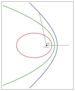
This can be shown to result in the trajectory being ideally a conic section (circle, ellipse, parabola or hyperbola) ^[10] with the central body located at one focus. Orbital trajectories are either circles or ellipses; the parabolic trajectory represents first escape of the vehicle from the central body's gravitational field. Hyperbolic trajectories are escape trajectories with excess velocity, and will be covered under Interplanetary flight below.

Elliptical orbits are characterized by three elements. ^[9] The semi-major axis a is the average of the radius at apoapsis and periapsis:

${\displaystyle a={\frac {r_{a}+r_{p}}{2}}}$

The eccentricity e can then be calculated for an ellipse, knowing the apses:

${\displaystyle e={\frac {r_{a}}{a}}-1}$

The time period for a complete orbit is dependent only on the semi-major axis, and is independent of eccentricity: ^[11]

${\displaystyle TP=2\pi {\sqrt {\frac {a^{3}}{\mu }}}\,}$

where ${\displaystyle \mu }$ is the standard gravitational parameter of the central body.

The angular orbital elements of a spacecraft orbiting a central body, defining orientation of the orbit in relation to its fundamental reference plane

The orientation of the orbit in space is specified by three angles:

• The inclinationi, of the orbital plane with the fundamental plane (this is usually a planet or moon's equatorial plane, or in the case of a solar orbit, the Earth's orbital plane around the Sun, known as the ecliptic.) Positive inclination is northward, while negative inclination is southward.
• The longitude of the ascending node Ω, measured in the fundamental plane counter-clockwise looking southward, from a reference direction (usually the vernal equinox) to the line where the spacecraft crosses this plane from south to north. (If inclination is zero, this angle is undefined and taken as 0.)
• The argument of periapsisω, measured in the orbital plane counter-clockwise looking southward, from the ascending node to the periapsis. If the inclination is 0, there is no ascending node, so ω is measured from the reference direction. For a circular orbit, there is no periapsis, so ω is taken as 0.

The orbital plane is ideally constant, but is usually subject to small perturbations caused by planetary oblateness and the presence of other bodies.

The spacecraft's position in orbit is specified by the true anomaly,${\displaystyle \nu }$, an angle measured from the periapsis, or for a circular orbit, from the ascending node or reference direction. The semi-latus rectum, or radius at 90 degrees from periapsis, is: ^[12]

${\displaystyle p=a(1-e^{2})\,}$

The radius at any position in flight is:

${\displaystyle r={\frac {p}{1+e\cos \nu }}\,}$

and the velocity at that position is:

${\displaystyle v={\sqrt {\mu \left({\frac {2}{r}}-{\frac {1}{a}}\right)}}\,}$

Types of orbit

Circular

For a circular orbit, r_a = r_p = a, and eccentricity is 0. Circular velocity at a given radius is:

${\displaystyle v_{c}={\sqrt {\frac {\mu }{r}}}\,}$

Elliptical

For an elliptical orbit, e is greater than 0 but less than 1. The periapsis velocity is:

${\displaystyle v_{p}={\sqrt {\frac {\mu (1+e)}{a(1-e)}}}\,}$

and the apoapsis velocity is:

${\displaystyle v_{a}={\sqrt {\frac {\mu (1-e)}{a(1+e)}}}\,}$

The limiting condition is a parabolic escape orbit, when e = 1 and r_a becomes infinite. Escape velocity at periapsis is then

${\displaystyle v_{e}={\sqrt {\frac {2\mu }{r_{p}}}}\,}$

Flight path angle

The specific angular momentum of any conic orbit, h, is constant, and is equal to the product of radius and velocity at periapsis. At any other point in the orbit, it is equal to: ^[13]

${\displaystyle h=rv\cos \varphi ,\,}$

where φ is the flight path angle measured from the local horizontal (perpendicular to r.) This allows the calculation of φ at any point in the orbit, knowing radius and velocity:

${\displaystyle \varphi =\arccos \left({\frac {r_{p}v_{p}}{rv}}\right)\,}$

Note that flight path angle is a constant 0 degrees (90 degrees from local vertical) for a circular orbit.

True anomaly as a function of time

It can be shown that the angular momentum equation given above also relates the rate of change in true anomaly to r, v, and φ, thus the true anomaly can be found as a function of time since periapsis passage by integration: ^[14]

${\displaystyle \nu =r_{p}v_{p}\int _{t_{p}}^{t}{\frac {1}{r^{2}}}\,dt}$

Conversely, the time required to reach a given anomaly is:

${\displaystyle t={\frac {1}{r_{p}v_{p}}}\int _{0}^{\nu }r^{2}\,d\nu }$

Orbital maneuvers

See also: Orbital maneuver

Once in orbit, a spacecraft may fire rocket engines to make in-plane changes to a different altitude or type of orbit, or to change its orbital plane. These maneuvers require changes in the craft's velocity, and the classical rocket equation is used to calculate the propellant requirements for a given delta-v. A delta-v budget will add up all the propellant requirements, or determine the total delta-v available from a given amount of propellant, for the mission. Most on-orbit maneuvers can be modeled as impulsive, that is as a near-instantaneous change in velocity, with minimal loss of accuracy.

In-plane changes

Orbit circularization

An elliptical orbit is most easily converted to a circular orbit at the periapsis or apoapsis by applying a single engine burn with a delta v equal to the difference between the desired orbit's circular velocity and the current orbit's periapsis or apoapsis velocity:

To circularize at periapsis, a retrograde burn is made:

${\displaystyle \Delta v\ =v_{c}-v_{p}\,}$

To circularize at apoapsis, a posigrade burn is made:

${\displaystyle \Delta v\ =v_{c}-v_{a}\,}$

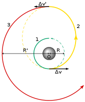
Altitude change by Hohmann transfer

Hohmann transfer orbit, 2, from an orbit (1) to a higher orbit (3)

A Hohmann transfer orbit is the simplest maneuver which can be used to move a spacecraft from one altitude to another. Two burns are required: the first to send the craft into the elliptical transfer orbit, and a second to circularize the target orbit.

To raise a circular orbit at ${\displaystyle v_{1}}$, the first posigrade burn raises velocity to the transfer orbit's periapsis velocity:

${\displaystyle \Delta v_{1}\ =v_{p}-v_{1}}$

The second posigrade burn, made at apoapsis, raises velocity to the target orbit's velocity:

${\displaystyle \Delta v_{2}\ =v_{2}-v_{a}}$

A maneuver to lower the orbit is the mirror image of the raise maneuver; both burns are made retrograde.

Altitude change by bi-elliptic transfer

A bi-elliptic transfer from a low circular starting orbit (dark blue) to a higher circular orbit (red)

A slightly more complicated altitude change maneuver is the bi-elliptic transfer, which consists of two half-elliptic orbits; the first, posigrade burn sends the spacecraft into an arbitrarily high apoapsis chosen at some point ${\displaystyle r_{b}}$ away from the central body. At this point a second burn modifies the periapsis to match the radius of the final desired orbit, where a third, retrograde burn is performed to inject the spacecraft into the desired orbit. ^[15] While this takes a longer transfer time, a bi-elliptic transfer can require less total propellant than the Hohmann transfer when the ratio of initial and target orbit radii is 12 or greater. ^{[16] [17]}

Burn 1 (posigrade):

${\displaystyle \Delta v_{1}\ ={v_{p}}_{1}-v_{1}}$

Burn 2 (posigrade or retrograde), to match periapsis to the target orbit's altitude:

${\displaystyle \Delta v_{2}\ ={v_{a}}_{2}-{v_{a}}_{1}}$

Burn 3 (retrograde):

${\displaystyle \Delta v_{3}\ =v_{2}-{v_{p}}_{2}}$

Change of plane

Plane change maneuvers can be performed alone or in conjunction with other orbit adjustments. For a pure rotation plane change maneuver, consisting only of a change in the inclination of the orbit, the specific angular momentum, h, of the initial and final orbits are equal in magnitude but not in direction. Therefore, the change in specific angular momentum can be written as:

${\displaystyle \Delta h=2h\sin \left({\frac {|\Delta i|}{2}}\right)}$

where h is the specific angular momentum before the plane change, and Δi is the desired change in the inclination angle. From this it can be shown ^[18] that the required delta-v is:

${\displaystyle \Delta v={\frac {2h\sin {\frac {|\Delta i|}{2}}}{r}}}$

From the definition of h, this can also be written as:

${\displaystyle \Delta v=2v\cos \varphi \sin \left({\frac {\left|\Delta i\right|}{2}}\right)}$

where v is the magnitude of velocity before plane change and φ is the flight path angle. Using the small-angle approximation, this becomes:

${\displaystyle \Delta v=v\cos(\varphi )\left|\Delta i\right|}$

The total delta-v for a combined maneuver can be calculated by a vector addition of the pure rotation delta-v and the delta-v for the other planned orbital change.

Translunar flight

A typical translunar trajectory

Vehicles sent on lunar or planetary missions are generally not launched by direct injection to departure trajectory, but first put into a low Earth parking orbit; this allows the flexibility of a bigger launch window and more time for checking that the vehicle is in proper condition for the flight.

Escape velocity is not required for flight to the Moon; rather the vehicle's apogee is raised high enough to take it through a point where it enters the Moon's gravitational sphere of influence (SOI). This is defined as the distance from a satellite at which its gravitational pull on a spacecraft equals that of its central body, which is

${\displaystyle r_{\text{SOI}}=D\left({\frac {m_{s}}{m_{c}}}\right)^{2/5},}$

where D is the mean distance from the satellite to the central body, and m_c and m_s are the masses of the central body and satellite, respectively. This value is approximately 66,300 kilometers (35,800 nautical miles) from Earth's Moon. ^[19]

An accurate solution of the trajectory requires treatment as a three-body problem, but a preliminary estimate may be made using a patched conic approximation of orbits around the Earth and Moon, patched at the SOI point and taking into account the fact that the Moon is a revolving frame of reference around the Earth.

Translunar injection

Main article: Translunar injection

This must be timed so that the Moon will be in position to capture the vehicle, and might be modeled to a first approximation as a Hohmann transfer. However, the rocket burn duration is usually long enough, and occurs during a sufficient change in flight path angle, that this is not very accurate. It must be modeled as a non-impulsive maneuver, requiring integration by finite element analysis of the accelerations due to propulsive thrust and gravity to obtain velocity and flight path angle: ^[7]

${\displaystyle {\dot {v}}={\frac {F\cos \alpha }{m}}-g\cos \theta \,}$

${\displaystyle {\dot {\theta }}={\frac {F\sin \alpha }{mv}}+\left({\frac {g}{v}}-{\frac {v}{r}}\right)\sin \theta ,\,}$

${\displaystyle v=\int _{t_{0}}^{t}{\dot {v}}\,dt}$

${\displaystyle \theta =\int _{t_{0}}^{t}{\dot {\theta }}\,dt}$

where:

F is the engine thrust;

α is the angle of attack;

m is the vehicle's mass;

r is the radial distance to the planet's center; and

g is the gravitational acceleration, which varies with the inverse square of the radial distance:

${\displaystyle g=g_{0}\left({\frac {r_{0}}{r}}\right)^{2}\,}$ ^[7]

Altitude ${\displaystyle h}$, downrange distance ${\displaystyle s}$, and radial distance ${\displaystyle r}$ from the center of the Earth are then computed as: ^[7]

${\displaystyle h=\int _{t_{0}}^{t}v\cos \theta \,dt}$

${\displaystyle r=r_{0}+h\,}$

${\displaystyle s=r_{0}\int _{t_{0}}^{t}{\frac {v}{r}}\sin \theta \,dt}$

Mid-course corrections

A simple lunar trajectory stays in one plane, resulting in lunar flyby or orbit within a small range of inclination to the Moon's equator. This also permits a "free return", in which the spacecraft would return to the appropriate position for reentry into the Earth's atmosphere if it were not injected into lunar orbit. Relatively small velocity changes are usually required to correct for trajectory errors. Such a trajectory was used for the Apollo 8, Apollo 10, Apollo 11, and Apollo 12 manned lunar missions.

Greater flexibility in lunar orbital or landing site coverage (at greater angles of lunar inclination) can be obtained by performing a plane change maneuver mid-flight; however, this takes away the free-return option, as the new plane would take the spacecraft's emergency return trajectory away from the Earth's atmospheric re-entry point, and leave the spacecraft in a high Earth orbit. This type of trajectory was used for the last five Apollo missions (13 through 17).

Lunar orbit insertion

In the Apollo program, the retrograde lunar orbit insertion burn was performed at an altitude of approximately 110 kilometers (59 nautical miles) on the far side of the Moon. This became the pericynthion of the initial orbits, with an apocynthion on the order of 300 kilometers (160 nautical miles). The delta v was approximately 1,000 meters per second (3,300 ft/s). Two orbits later, the orbit was circularized at 110 kilometers (59 nautical miles). ^[20] For each mission, the flight dynamics officer prepared 10 lunar orbit insertion solutions so the one could be chosen with the optimum (minimum) fuel burn and best met the mission requirements; this was uploaded to the spacecraft computer and had to be executed and monitored by the astronauts on the lunar far side, while they were out of radio contact with Earth. ^[20]

Interplanetary flight

In order to completely leave one planet's gravitational field to reach another, a hyperbolic trajectory relative to the departure planet is necessary, with excess velocity added to (or subtracted from) the departure planet's orbital velocity around the Sun. The desired heliocentric transfer orbit to a superior planet will have its perihelion at the departure planet, requiring the hyperbolic excess velocity to be applied in the posigrade direction, when the spacecraft is away from the Sun. To an inferior planet destination, aphelion will be at the departure planet, and the excess velocity is applied in the retrograde direction when the spacecraft is toward the Sun. For accurate mission calculations, the orbital elements of the planets must be obtained from an ephemeris, ^[21] such as that published by NASA's Jet Propulsion Laboratory.

Simplifying assumptions

Body	Eccentricity [22]	Mean distance 106 km [23]	Orbital speed km/sec [23]	Orbital period years [23]	Mass Earth = 1 [23]	${\displaystyle \mu }$ km3/sec2 [23]
Sun	---	---	---	---	333,432	1.327x1011
Mercury	.2056	57.9	47.87	.241	.056	2.232x104
Venus	.0068	108.1	35.04	.615	.817	3.257x105
Earth	.0167	149.5	29.79	1.000	1.000	3.986x105
Mars	.0934	227.8	24.14	1.881	.108	4.305x104
Jupiter	.0484	778	13.06	11.86	318.0	1.268x108
Saturn	.0541	1426	9.65	29.46	95.2	3.795x107
Uranus	.0472	2868	6.80	84.01	14.6	5.820x106
Neptune	.0086	4494	5.49	164.8	17.3	6.896x106

For the purpose of preliminary mission analysis and feasibility studies, certain simplified assumptions may be made to enable delta-v calculation with very small error: ^[24]

• All the planets' orbits except Mercury have very small eccentricity, and therefore may be assumed to be circular at a constant orbital speed and mean distance from the Sun.
• All the planets' orbits (except Mercury) are nearly coplanar, with very small inclination to the ecliptic (3.39 degrees or less; Mercury's inclination is 7.00 degrees).
• The perturbating effects of the other planets' gravity is negligible.
• The spacecraft will spend most of its flight time under only the gravitational influence of the Sun, except for brief periods when it is in the sphere of influence of the departure and destination planets.

Since interplanetary spacecraft spend a large period of time in heliocentric orbit between the planets, which are at relatively large distances away from each other, the patched-conic approximation is much more accurate for interplanetary trajectories than for translunar trajectories. ^[24] The patch point between the hyperbolic trajectory relative to the departure planet and the heliocentric transfer orbit occurs at the planet's sphere of influence radius relative to the Sun, as defined above in Orbital flight. Given the Sun's mass ratio of 333,432 times that of Earth and distance of 149,500,000 kilometers (80,700,000 nautical miles), the Earth's sphere of influence radius is 924,000 kilometers (499,000 nautical miles) (roughly 1,000,000 kilometers). ^[25]

Heliocentric transfer orbit

The transfer orbit required to carry the spacecraft from the departure planet's orbit to the destination planet is chosen among several options:

• A Hohmann transfer orbit requires the least possible propellant and delta-v; this is half of an elliptical orbit with aphelion and perihelion tangential to both planets' orbits, with the longest outbound flight time equal to half the period of the ellipse. This is known as a conjunction-class mission. ^{[26] [27]} There is no "free return" option, because if the spacecraft does not enter orbit around the destination planet and instead completes the transfer orbit, the departure planet will not be in its original position. Using another Hohmann transfer to return requires a significant loiter time at the destination planet, resulting in a very long total round-trip mission time. ^[28] Science fiction writer Arthur C. Clarke wrote in his 1951 book The Exploration of Space that an Earth-to-Mars round trip would require 259 days outbound and another 259 days inbound, with a 425-day stay at Mars.
• Increasing the departure apsis speed (and thus the semi-major axis) results in a trajectory which crosses the destination planet's orbit non-tangentially before reaching the opposite apsis, increasing delta-v but cutting the outbound transit time below the maximum. ^[28]
• A gravity assist maneuver, sometimes known as a "slingshot maneuver" or Crocco mission after its 1956 proposer Gaetano Crocco, results in an opposition-class mission with a much shorter dwell time at the destination. ^{[29] [27]} This is accomplished by swinging past another planet, using its gravity to alter the orbit. A round trip to Mars, for example, can be significantly shortened from the 943 days required for the conjunction mission, to under a year, by swinging past Venus on return to the Earth.

Hyperbolic departure

The required hyperbolic excess velocity v_∞ (sometimes called characteristic velocity) is the difference between the transfer orbit's departure speed and the departure planet's heliocentric orbital speed. Once this is determined, the injection velocity relative to the departure planet at periapsis is: ^[30]

${\displaystyle v_{p}={\sqrt {{\frac {2\mu }{r_{p}}}+v_{\infty }^{2}}}\,}$

The excess velocity vector for a hyperbola is displaced from the periapsis tangent by a characteristic angle, therefore the periapsis injection burn must lead the planetary departure point by the same angle: ^[31]

${\displaystyle \delta =\arcsin {\frac {1}{e}}\,}$

The geometric equation for eccentricity of an ellipse cannot be used for a hyperbola. But the eccentricity can be calculated from dynamics formulations as: ^[32]

${\displaystyle e={\sqrt {1+{\frac {2\varepsilon h^{2}}{\mu ^{2}}}}},}$

where h is the specific angular momentum as given above in the Orbital flight section, calculated at the periapsis: ^[31]

${\displaystyle h=r_{p}v_{p},\,}$

and ε is the specific energy: ^[31]

${\displaystyle \varepsilon ={\frac {v^{2}}{2}}-{\frac {\mu }{r}}\,}$

Also, the equations for r and v given in Orbital flight depend on the semi-major axis, and thus are unusable for an escape trajectory. But setting radius at periapsis equal to the r equation at zero anomaly gives an alternate expression for the semi-latus rectum:

${\displaystyle p=r_{p}(1+e),\,}$

which gives a more general equation for radius versus anomaly which is usable at any eccentricity:

${\displaystyle r={\frac {r_{p}(1+e)}{1+e\cos \nu }}\,}$

Substituting the alternate expression for p also gives an alternate expression for a (which is defined for a hyperbola, but no longer represents the semi-major axis). This gives an equation for velocity versus radius which is likewise usable at any eccentricity:

${\displaystyle v={\sqrt {\mu \left({\frac {2}{r}}-{\frac {(1-e^{2})}{r_{p}(1+e)}}\right)}}\,}$

The equations for flight path angle and anomaly versus time given in Orbital flight are also usable for hyperbolic trajectories.

Launch windows

There is a great deal of variation with time of the velocity change required for a mission, because of the constantly varying relative positions of the planets. Therefore, optimum launch windows are often chosen from the results of porkchop plots that show contours of characteristic energy (v_∞²) plotted versus departure and arrival time.

Atmospheric entry

Main article: Atmospheric entry

Controlled entry, descent, and landing of a vehicle is achieved by shedding the excess kinetic energy through aerodynamic heating from drag, which requires some means of heat shielding, and/or retrograde thrust. Terminal descent is usually achieved by means of parachutes and/or air brakes.

Attitude control

Main article: Attitude control

Since spacecraft spend most of their flight time coasting unpowered through the vacuum of space, they are unlike aircraft in that their flight trajectory is not determined by their attitude (orientation), except during atmospheric flight to control the forces of lift and drag, and during powered flight to align the thrust vector. Nonetheless, attitude control is often maintained in unpowered flight to keep the spacecraft in a fixed orientation for purposes of astronomical observation, communications, or for solar power generation; or to place it into a controlled spin for passive thermal control, or to create artificial gravity inside the craft.

Attitude control is maintained with respect to an inertial frame of reference or another entity (the celestial sphere, certain fields, nearby objects, etc.). The attitude of a craft is described by angles relative to three mutually perpendicular axes of rotation, referred to as roll, pitch, and yaw. Orientation can be determined by calibration using an external guidance system, such as determining the angles to a reference star or the Sun, then internally monitored using an inertial system of mechanical or optical gyroscopes. Orientation is a vector quantity described by three angles for the instantaneous direction, and the instantaneous rates of roll in all three axes of rotation. The aspect of control implies both awareness of the instantaneous orientation and rates of roll and the ability to change the roll rates to assume a new orientation using either a reaction control system or other means.

Newton's second law, applied to rotational rather than linear motion, becomes: ^[33]

${\displaystyle \mathbf {\tau _{x}} =I_{x}\mathbf {\alpha _{x}} ,}$

where ${\displaystyle \mathbf {\tau _{x}} }$ is the net torque about an axis of rotation exerted on the vehicle, I_x is its moment of inertia about that axis (a physical property that combines the mass and its distribution around the axis), and ${\displaystyle {alpha_{x}}}$ is the angular acceleration about that axis in radians per second per second. Therefore, the acceleration rate in degrees per second per second is

${\displaystyle \mathbf {\alpha _{x}} =(180/\pi )\mathbf {\tau _{x}} /I_{x},}$

Analogous to linear motion, the angular rotation rate ${\displaystyle \mathbf {\omega _{x}} }$ (degrees per second) is obtained by integrating α over time:

${\displaystyle {\omega _{x}}=\int _{t_{0}}^{t}{\alpha _{x}}dt}$

and the angular rotation ${\displaystyle \mathbf {\theta _{x}} }$ is the time integral of the rate:

${\displaystyle \theta _{x}=\int _{t_{0}}^{t}{\omega _{x}}dt}$

The three principal moments of inertia I_x, I_y, and I_z about the roll, pitch and yaw axes, are determined through the vehicle's center of mass.

The control torque for a launch vehicle is sometimes provided aerodynamically by movable fins, and usually by mounting the engines on gimbals to vector the thrust around the center of mass. Torque is frequently applied to spacecraft, operating absent aerodynamic forces, by a reaction control system, a set of thrusters located about the vehicle. The thrusters are fired, either manually or under automatic guidance control, in short bursts to achieve the desired rate of rotation, and then fired in the opposite direction to halt rotation at the desired position. The torque about a specific axis is:

${\displaystyle \mathbf {\tau } =\sum _{i=1}^{N}(r_{i}\times \mathbf {F_{i}} ),}$

where r is its distance from the center of mass, and F is the thrust of an individual thruster (only the component of F perpendicular to r is included.)

For situations where propellant consumption may be a problem (such as long-duration satellites or space stations), alternative means may be used to provide the control torque, such as reaction wheels ^[34] or control moment gyroscopes. ^[35]

Notes

1. "ESA - Flight Dynamics". European Space Agency. Retrieved June 22, 2020.
2. Bate, Mueller & White (1971), pp. 11–12.
3. George P. Sutton & Oscar Biblarz (2001). Rocket Propulsion Elements (7th ed.). Wiley Interscience. ISBN   0-471-32642-9. See Equation 2-14.
4. Sutton, George P.; Biblarz, Oscar (2001). Rocket Propulsion Elements. John Wiley & Sons. ISBN   978-0-471-32642-7. Archived from the original on 12 January 2014. Retrieved 28 May 2016.
5. George P. Sutton & Oscar Biblarz (2001). Rocket Propulsion Elements (7th ed.). Wiley Interscience. ISBN   0-471-32642-9. See Equation 3-33.
6. Anderson (2004), pp. 257–261.
7. Kromis (1967), p. 11:154.
8. Glasstone (1965), p. 209, §4.97.
9. Perry (1967), p. 11:151.
10. Bate, Mueller & White (1971), pp. 11–40.
11. Bate, Mueller & White (1971), p. 33.
12. Bate, Mueller & White (1971), p. 24.
13. Bate, Mueller & White (1971), p. 18.
14. Bate, Mueller & White (1971), pp. 31–32.
15. Curtis, Howard (2005). Orbital Mechanics for Engineering Students. Elsevier. p. 264. ISBN   0-7506-6169-0.
16. Gobetz, F. W.; Doll, J. R. (May 1969). "A Survey of Impulsive Trajectories". AIAA Journal. American Institute of Aeronautics and Astronautics. 7 (5): 801–834. Bibcode:1969AIAAJ...7..801D. doi:10.2514/3.5231.
17. Escobal, Pedro R. (1968). Methods of Astrodynamics. New York: John Wiley & Sons. ISBN   978-0-471-24528-5.
18. Hintz (2015), p. 112.
19. Bate, Mueller & White (1971), pp. 333–334.
20. O'Brien, Frank (1999). "Lunar Orbit Insertion". Apollo Flight Journal. David Woods. Retrieved June 25, 2020.
21. Bate, Mueller & White (1971), p. 359.
22. "Keplerian elements for 1800 A.D. to 2050 A.D." JPL Solar System Dynamics. Retrieved 17 December 2009.
23. Bate, Mueller & White (1971), p. 361.
24. Bate, Mueller & White (1971), pp. 359, 362.
25. Bate, Mueller & White (1971), p. 368.
26. Mattfeld et al. (2015), p. 3.
27. Drake et al. 2017.
28. Bate, Mueller & White (1971), pp. 362–363.
29. Mattfeld et al. (2015), pp. 3–4.
30. Bate, Mueller & White (1971), p. 369.
31. Bate, Mueller & White (1971), p. 371.
32. Bate, Mueller & White (1971), p. 372.
33. Beer & Johnston (1972), p. 499.
34. "Reaction/Momentum Wheel". NASA. Retrieved 15 June 2018.
35. Gurrisi, Charles; Seidel, Raymond; Dickerson, Scott; Didziulis, Stephen; Frantz, Peter; Ferguson, Kevin (12 May 2010). "Space Station Control Moment Gyroscope Lessons Learned" (PDF). Proceedings of the 40th Aerospace Mechanisms Symposium.

References

• Anderson, John D. (2004), Introduction to Flight (5th ed.), McGraw-Hill, ISBN   0-07-282569-3
• Bate, Roger B.; Mueller, Donald D.; White, Jerry E. (1971), Fundamentals of Astrodynamics, Dover
• Beer, Ferdinand P.; Johnston, Russell, Jr. (1972), Vector Mechanics for Engineers: Statics & Dynamics, McGraw-Hill
• Drake, Bret G.; Baker, John D.; Hoffman, Stephan J.; Landau, Damon; Voels, Stephen A. (2017). "Trajectory Options for Exploring Mars and the Moons of Mars". NASA Human Spaceflight Architecture Team (Presentation).
• Fellenz, D.W. (1967). "Atmospheric Entry". In Theodore Baumeister (ed.). Marks' Standard Handbook for Mechanical Engineers (Seventh ed.). New York City: McGraw Hill. pp. 11:155–58. ISBN   0-07-142867-4.
• Glasstone, Samuel (1965). Sourcebook on the Space Sciences. D. Van Nostrand Company, Inc.
• Hintz, Gerald R. (2015). Orbital Mechanics and Astrodynamics: Techniques and Tools for Space Missions. Cham. ISBN   9783319094441. OCLC   900730410.
• Kromis, A.J. (1967). "Powered-Flight-Trajectory Analysis". In Theodore Baumeister (ed.). Marks' Standard Handbook for Mechanical Engineers (Seventh ed.). New York City: McGraw Hill. pp. 11:154–55. ISBN   0-07-142867-4.
• Mattfeld, Bryan; Stromgren, Chel; Shyface, Hilary; Komar, David R.; Cirillo, William; Goodliff, Kandyce (2015). "Trades Between Opposition and Conjunction Class Trajectories for Early Human Missions to Mars" (PDF). Retrieved July 10, 2018.
• Perry, W.R. (1967). "Orbital Mechanics". In Theodore Baumeister (ed.). Marks' Standard Handbook for Mechanical Engineers (Seventh ed.). New York City: McGraw Hill. pp. 11:151–52. ISBN   0-07-142867-4.
• Russell, J.W. (1967). "Lunar and Interplanetary Flight Mechanics". In Theodore Baumeister (ed.). Marks' Standard Handbook for Mechanical Engineers (Seventh ed.). New York City: McGraw Hill. pp. 11:152–54. ISBN   0-07-142867-4.
• Sidi, M.J. "Spacecraft Dynamics & Control. Cambridge, 1997.
• Thomson, W.T. "Introduction to Space Dynamics." Dover, 1961.
• Wertz, J.R. "Spacecraft Attitude Determination and Control." Kluwer, 1978.
• Wiesel, W.E. "Spaceflight Dynamics." McGraw-Hill, 1997.