In probability theory, Chebyshev's inequality guarantees that, for a wide class of probability distributions, no more than a certain fraction of values can be more than a certain distance from the mean. Specifically, no more than 1/k2 of the distribution's values can be k or more standard deviations away from the mean. The rule is often called Chebyshev's theorem, about the range of standard deviations around the mean, in statistics. The inequality has great utility because it can be applied to any probability distribution in which the mean and variance are defined. For example, it can be used to prove the weak law of large numbers.

In statistics, a multimodaldistribution is a probability distribution with more than one mode. These appear as distinct peaks in the probability density function, as shown in Figures 1 and 2. Categorical, continuous, and discrete data can all form multimodal distributions. Among univariate analyses, multimodal distributions are commonly bimodal.
In probability theory and statistics, the generalized extreme value (GEV) distribution is a family of continuous probability distributions developed within extreme value theory to combine the Gumbel, Fréchet and Weibull families also known as type I, II and III extreme value distributions. By the extreme value theorem the GEV distribution is the only possible limit distribution of properly normalized maxima of a sequence of independent and identically distributed random variables. Note that a limit distribution needs to exist, which requires regularity conditions on the tail of the distribution. Despite this, the GEV distribution is often used as an approximation to model the maxima of long (finite) sequences of random variables.
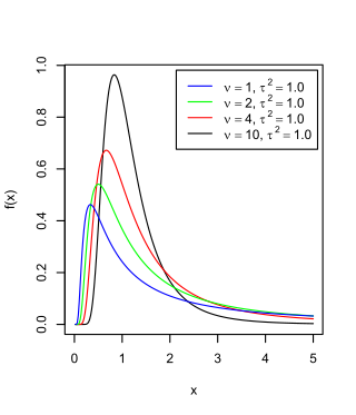
The scaled inverse chi-squared distribution is the distribution for x = 1/s2, where s2 is a sample mean of the squares of ν independent normal random variables that have mean 0 and inverse variance 1/σ2 = τ2. The distribution is therefore parametrised by the two quantities ν and τ2, referred to as the number of chi-squared degrees of freedom and the scaling parameter, respectively.

The Pearson distribution is a family of continuous probability distributions. It was first published by Karl Pearson in 1895 and subsequently extended by him in 1901 and 1916 in a series of articles on biostatistics.
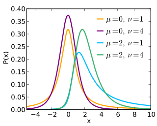
The noncentral t-distribution generalizes Student's t-distribution using a noncentrality parameter. Whereas the central probability distribution describes how a test statistic t is distributed when the difference tested is null, the noncentral distribution describes how t is distributed when the null is false. This leads to its use in statistics, especially calculating statistical power. The noncentral t-distribution is also known as the singly noncentral t-distribution, and in addition to its primary use in statistical inference, is also used in robust modeling for data.

The folded normal distribution is a probability distribution related to the normal distribution. Given a normally distributed random variable X with mean μ and variance σ2, the random variable Y = |X| has a folded normal distribution. Such a case may be encountered if only the magnitude of some variable is recorded, but not its sign. The distribution is called "folded" because probability mass to the left of x = 0 is folded over by taking the absolute value. In the physics of heat conduction, the folded normal distribution is a fundamental solution of the heat equation on the half space; it corresponds to having a perfect insulator on a hyperplane through the origin.
Bayesian linear regression is a type of conditional modeling in which the mean of one variable is described by a linear combination of other variables, with the goal of obtaining the posterior probability of the regression coefficients and ultimately allowing the out-of-sample prediction of the regressandconditional on observed values of the regressors. The simplest and most widely used version of this model is the normal linear model, in which given is distributed Gaussian. In this model, and under a particular choice of prior probabilities for the parameters—so-called conjugate priors—the posterior can be found analytically. With more arbitrarily chosen priors, the posteriors generally have to be approximated.
Expected shortfall (ES) is a risk measure—a concept used in the field of financial risk measurement to evaluate the market risk or credit risk of a portfolio. The "expected shortfall at q% level" is the expected return on the portfolio in the worst of cases. ES is an alternative to value at risk that is more sensitive to the shape of the tail of the loss distribution.
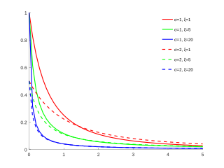
In statistics, the generalized Pareto distribution (GPD) is a family of continuous probability distributions. It is often used to model the tails of another distribution. It is specified by three parameters: location , scale , and shape . Sometimes it is specified by only scale and shape and sometimes only by its shape parameter. Some references give the shape parameter as .
In financial mathematics, tail value at risk (TVaR), also known as tail conditional expectation (TCE) or conditional tail expectation (CTE), is a risk measure associated with the more general value at risk. It quantifies the expected value of the loss given that an event outside a given probability level has occurred.
The Birnbaum–Saunders distribution, also known as the fatigue life distribution, is a probability distribution used extensively in reliability applications to model failure times. There are several alternative formulations of this distribution in the literature. It is named after Z. W. Birnbaum and S. C. Saunders.

The shifted log-logistic distribution is a probability distribution also known as the generalized log-logistic or the three-parameter log-logistic distribution. It has also been called the generalized logistic distribution, but this conflicts with other uses of the term: see generalized logistic distribution.
The term generalized logistic distribution is used as the name for several different families of probability distributions. For example, Johnson et al. list four forms, which are listed below.

In probability theory and statistics, the half-normal distribution is a special case of the folded normal distribution.

In probability theory and statistics, the skew normal distribution is a continuous probability distribution that generalises the normal distribution to allow for non-zero skewness.

In probability theory and statistics, the normal-inverse-gamma distribution is a four-parameter family of multivariate continuous probability distributions. It is the conjugate prior of a normal distribution with unknown mean and variance.

In probability theory and statistics, the generalized chi-squared distribution is the distribution of a quadratic form of a multinormal variable, or a linear combination of different normal variables and squares of normal variables. Equivalently, it is also a linear sum of independent noncentral chi-square variables and a normal variable. There are several other such generalizations for which the same term is sometimes used; some of them are special cases of the family discussed here, for example the gamma distribution.
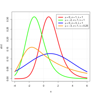
In probability theory, an exponentially modified Gaussian distribution describes the sum of independent normal and exponential random variables. An exGaussian random variable Z may be expressed as Z = X + Y, where X and Y are independent, X is Gaussian with mean μ and variance σ2, and Y is exponential of rate λ. It has a characteristic positive skew from the exponential component.
In statistics and probability theory, the nonparametric skew is a statistic occasionally used with random variables that take real values. It is a measure of the skewness of a random variable's distribution—that is, the distribution's tendency to "lean" to one side or the other of the mean. Its calculation does not require any knowledge of the form of the underlying distribution—hence the name nonparametric. It has some desirable properties: it is zero for any symmetric distribution; it is unaffected by a scale shift; and it reveals either left- or right-skewness equally well. In some statistical samples it has been shown to be less powerful than the usual measures of skewness in detecting departures of the population from normality.


