
A random variable is a mathematical formalization of a quantity or object which depends on random events. The term 'random variable' can be misleading as its mathematical definition is not actually random nor a variable, but rather it is a function from possible outcomes in a sample space to a measurable space, often to the real numbers.
Independence is a fundamental notion in probability theory, as in statistics and the theory of stochastic processes. Two events are independent, statistically independent, or stochastically independent if, informally speaking, the occurrence of one does not affect the probability of occurrence of the other or, equivalently, does not affect the odds. Similarly, two random variables are independent if the realization of one does not affect the probability distribution of the other.
In probability, and statistics, a multivariate random variable or random vector is a list or vector of mathematical variables each of whose value is unknown, either because the value has not yet occurred or because there is imperfect knowledge of its value. The individual variables in a random vector are grouped together because they are all part of a single mathematical system — often they represent different properties of an individual statistical unit. For example, while a given person has a specific age, height and weight, the representation of these features of an unspecified person from within a group would be a random vector. Normally each element of a random vector is a real number.

In probability theory and statistics, the multivariate normal distribution, multivariate Gaussian distribution, or joint normal distribution is a generalization of the one-dimensional (univariate) normal distribution to higher dimensions. One definition is that a random vector is said to be k-variate normally distributed if every linear combination of its k components has a univariate normal distribution. Its importance derives mainly from the multivariate central limit theorem. The multivariate normal distribution is often used to describe, at least approximately, any set of (possibly) correlated real-valued random variables each of which clusters around a mean value.
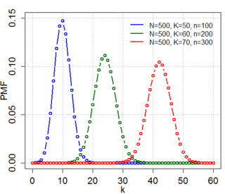
In probability theory and statistics, the hypergeometric distribution is a discrete probability distribution that describes the probability of successes in draws, without replacement, from a finite population of size that contains exactly objects with that feature, wherein each draw is either a success or a failure. In contrast, the binomial distribution describes the probability of successes in draws with replacement.
In mathematics, an indicator function or a characteristic function of a subset of a set is a function that maps elements of the subset to one, and all other elements to zero. That is, if A is a subset of some set X, then if and otherwise, where is a common notation for the indicator function. Other common notations are and
In statistics, the Wishart distribution is a generalization of the gamma distribution to multiple dimensions. It is named in honor of John Wishart, who first formulated the distribution in 1928. Other names include Wishart ensemble, or Wishart–Laguerre ensemble, or LOE, LUE, LSE.
In mathematics, the total variation identifies several slightly different concepts, related to the (local or global) structure of the codomain of a function or a measure. For a real-valued continuous function f, defined on an interval [a, b] ⊂ R, its total variation on the interval of definition is a measure of the one-dimensional arclength of the curve with parametric equation x ↦ f(x), for x ∈ [a, b]. Functions whose total variation is finite are called functions of bounded variation.
Importance sampling is a Monte Carlo method for evaluating properties of a particular distribution, while only having samples generated from a different distribution than the distribution of interest. Its introduction in statistics is generally attributed to a paper by Teun Kloek and Herman K. van Dijk in 1978, but its precursors can be found in statistical physics as early as 1949. Importance sampling is also related to umbrella sampling in computational physics. Depending on the application, the term may refer to the process of sampling from this alternative distribution, the process of inference, or both.

Given two random variables that are defined on the same probability space, the joint probability distribution is the corresponding probability distribution on all possible pairs of outputs. The joint distribution can just as well be considered for any given number of random variables. The joint distribution encodes the marginal distributions, i.e. the distributions of each of the individual random variables and the conditional probability distributions, which deal with how the outputs of one random variable are distributed when given information on the outputs of the other random variable(s).

In probability and statistics, the Dirichlet distribution (after Peter Gustav Lejeune Dirichlet), often denoted , is a family of continuous multivariate probability distributions parameterized by a vector of positive reals. It is a multivariate generalization of the beta distribution, hence its alternative name of multivariate beta distribution (MBD). Dirichlet distributions are commonly used as prior distributions in Bayesian statistics, and in fact, the Dirichlet distribution is the conjugate prior of the categorical distribution and multinomial distribution.
In statistics, generalized least squares (GLS) is a method used to estimate the unknown parameters in a linear regression model. It is used when there is a non-zero amount of correlation between the residuals in the regression model. GLS is employed to improve statistical efficiency and reduce the risk of drawing erroneous inferences, as compared to conventional least squares and weighted least squares methods. It was first described by Alexander Aitken in 1935.
In probability theory and statistics, partial correlation measures the degree of association between two random variables, with the effect of a set of controlling random variables removed. When determining the numerical relationship between two variables of interest, using their correlation coefficient will give misleading results if there is another confounding variable that is numerically related to both variables of interest. This misleading information can be avoided by controlling for the confounding variable, which is done by computing the partial correlation coefficient. This is precisely the motivation for including other right-side variables in a multiple regression; but while multiple regression gives unbiased results for the effect size, it does not give a numerical value of a measure of the strength of the relationship between the two variables of interest.
In probability theory and statistics, the Dirichlet-multinomial distribution is a family of discrete multivariate probability distributions on a finite support of non-negative integers. It is also called the Dirichlet compound multinomial distribution (DCM) or multivariate Pólya distribution. It is a compound probability distribution, where a probability vector p is drawn from a Dirichlet distribution with parameter vector , and an observation drawn from a multinomial distribution with probability vector p and number of trials n. The Dirichlet parameter vector captures the prior belief about the situation and can be seen as a pseudocount: observations of each outcome that occur before the actual data is collected. The compounding corresponds to a Pólya urn scheme. It is frequently encountered in Bayesian statistics, machine learning, empirical Bayes methods and classical statistics as an overdispersed multinomial distribution.
In probability and statistics, a natural exponential family (NEF) is a class of probability distributions that is a special case of an exponential family (EF).
In statistics, the hypergeometric distribution is the discrete probability distribution generated by picking colored balls at random from an urn without replacement.

In probability theory and statistics, Fisher's noncentral hypergeometric distribution is a generalization of the hypergeometric distribution where sampling probabilities are modified by weight factors. It can also be defined as the conditional distribution of two or more binomially distributed variables dependent upon their fixed sum.
When an electromagnetic wave travels through a medium in which it gets attenuated, it undergoes exponential decay as described by the Beer–Lambert law. However, there are many possible ways to characterize the wave and how quickly it is attenuated. This article describes the mathematical relationships among:
In statistics, the matrix t-distribution is the generalization of the multivariate t-distribution from vectors to matrices. The matrix t-distribution shares the same relationship with the multivariate t-distribution that the matrix normal distribution shares with the multivariate normal distribution. For example, the matrix t-distribution is the compound distribution that results from sampling from a matrix normal distribution having sampled the covariance matrix of the matrix normal from an inverse Wishart distribution.
In probability theory and statistics, the Dirichlet negative multinomial distribution is a multivariate distribution on the non-negative integers. It is a multivariate extension of the beta negative binomial distribution. It is also a generalization of the negative multinomial distribution (NM(k, p)) allowing for heterogeneity or overdispersion to the probability vector. It is used in quantitative marketing research to flexibly model the number of household transactions across multiple brands.


