In probability theory, Chebyshev's inequality (also called the Bienaymé–Chebyshev inequality) provides an upper bound on the probability of deviation of a random variable (with finite variance) from its mean. More specifically, the probability that a random variable deviates from its mean by more than is at most , where is any positive constant and is the standard deviation (the square root of the variance).
The rule is often called Chebyshev's theorem, about the range of standard deviations around the mean, in statistics. The inequality has great utility because it can be applied to any probability distribution in which the mean and variance are defined. For example, it can be used to prove the weak law of large numbers.
Its practical usage is similar to the 68–95–99.7 rule, which applies only to normal distributions. Chebyshev's inequality is more general, stating that a minimum of just 75% of values must lie within two standard deviations of the mean and 88.89% within three standard deviations for a broad range of different probability distributions. [1] [2]
The term Chebyshev's inequality may also refer to Markov's inequality, especially in the context of analysis. They are closely related, and some authors refer to Markov's inequality as "Chebyshev's First Inequality," and the similar one referred to on this page as "Chebyshev's Second Inequality."
Chebyshev's inequality is tight in the sense that for each chosen positive constant, there exists a random variable such that the inequality is in fact an equality. [3]
The theorem is named after Russian mathematician Pafnuty Chebyshev, although it was first formulated by his friend and colleague Irénée-Jules Bienaymé. [4] : 98 The theorem was first proved by Bienaymé in 1853 [5] and more generally proved by Chebyshev in 1867. [6] [7] His student Andrey Markov provided another proof in his 1884 Ph.D. thesis. [8]
Chebyshev's inequality is usually stated for random variables, but can be generalized to a statement about measure spaces.
Let X (integrable) be a random variable with finite non-zero variance σ2 (and thus finite expected value μ). [9] Then for any real number k > 0,
Only the case is useful. When the right-hand side and the inequality is trivial as all probabilities are ≤ 1.
As an example, using shows that the probability values lie outside the interval does not exceed . Equivalently, it implies that the probability of values lying within the interval (i.e. its "coverage") is at least.
Because it can be applied to completely arbitrary distributions provided they have a known finite mean and variance, the inequality generally gives a poor bound compared to what might be deduced if more aspects are known about the distribution involved.
k | Min. % within k standard deviations of mean | Max. % beyond k standard deviations from mean |
---|---|---|
1 | 0% | 100% |
√2 | 50% | 50% |
1.5 | 55.56% | 44.44% |
2 | 75% | 25% |
2√2 | 87.5% | 12.5% |
3 | 88.8889% | 11.1111% |
4 | 93.75% | 6.25% |
5 | 96% | 4% |
6 | 97.2222% | 2.7778% |
7 | 97.9592% | 2.0408% |
8 | 98.4375% | 1.5625% |
9 | 98.7654% | 1.2346% |
10 | 99% | 1% |
Let (X, Σ, μ) be a measure space, and let f be an extended real-valued measurable function defined on X. Then for any real number t > 0 and 0 < p < ∞,
More generally, if g is an extended real-valued measurable function, nonnegative and nondecreasing, with then: [ citation needed ]
This statement follows from the Markov inequality, , with and , since in this case . The previous statement then follows by defining as if and otherwise.
Suppose we randomly select a journal article from a source with an average of 1000 words per article, with a standard deviation of 200 words. We can then infer that the probability that it has between 600 and 1400 words (i.e. within standard deviations of the mean) must be at least 75%, because there is no more than chance to be outside that range, by Chebyshev's inequality. But if we additionally know that the distribution is normal, we can say there is a 75% chance the word count is between 770 and 1230 (which is an even tighter bound).
As shown in the example above, the theorem typically provides rather loose bounds. However, these bounds cannot in general (remaining true for arbitrary distributions) be improved upon. The bounds are sharp for the following example: for any k ≥ 1,
For this distribution, the mean μ = 0 and the variance σ2 = (−1)2/2k2 + 0 + 12/2k2 = 1/k2, so the standard deviation σ = 1/k and
Chebyshev's inequality is an equality for precisely those distributions which are affine transformations of this example.
Markov's inequality states that for any real-valued random variable Y and any positive number a, we have . One way to prove Chebyshev's inequality is to apply Markov's inequality to the random variable with :
It can also be proved directly using conditional expectation:
Chebyshev's inequality then follows by dividing by k2σ2. This proof also shows why the bounds are quite loose in typical cases: the conditional expectation on the event where |X − μ| < kσ is thrown away, and the lower bound of k2σ2 on the event |X − μ| ≥ kσ can be quite poor.
Chebyshev's inequality can also be obtained directly from a simple comparison of areas, starting from the representation of an expected value as the difference of two improper Riemann integrals (last formula in the definition of expected value for arbitrary real-valued random variables). [10]
Several extensions of Chebyshev's inequality have been developed.
Selberg derived a generalization to arbitrary intervals. [11] Suppose X is a random variable with mean μ and variance σ2. Selberg's inequality states [12] that if ,
When , this reduces to Chebyshev's inequality. These are known to be the best possible bounds. [13]
Chebyshev's inequality naturally extends to the multivariate setting, where one has n random variables Xi with mean μi and variance σi2. Then the following inequality holds.
This is known as the Birnbaum–Raymond–Zuckerman inequality after the authors who proved it for two dimensions. [14] This result can be rewritten in terms of vectors X = (X1, X2, ...) with mean μ = (μ1, μ2, ...), standard deviation σ = (σ1, σ2, ...), in the Euclidean norm || ⋅ ||. [15]
One can also get a similar infinite-dimensional Chebyshev's inequality. A second related inequality has also been derived by Chen. [16] Let n be the dimension of the stochastic vector X and let E(X) be the mean of X. Let S be the covariance matrix and k > 0. Then
where YT is the transpose of Y. The inequality can be written in terms of the Mahalanobis distance as
where the Mahalanobis distance based on S is defined by
Navarro [17] proved that these bounds are sharp, that is, they are the best possible bounds for that regions when we just know the mean and the covariance matrix of X.
Stellato et al. [18] showed that this multivariate version of the Chebyshev inequality can be easily derived analytically as a special case of Vandenberghe et al. [19] where the bound is computed by solving a semidefinite program (SDP).
If the variables are independent this inequality can be sharpened. [20]
Berge derived an inequality for two correlated variables X1, X2. [21] Let ρ be the correlation coefficient between X1 and X2 and let σi2 be the variance of Xi. Then
This result can be sharpened to having different bounds for the two random variables [22] and having asymmetric bounds, as in Selberg's inequality. [23]
Olkin and Pratt derived an inequality for n correlated variables. [24]
where the sum is taken over the n variables and
where ρij is the correlation between Xi and Xj.
Olkin and Pratt's inequality was subsequently generalised by Godwin. [25]
Mitzenmacher and Upfal [26] note that by applying Markov's inequality to the nonnegative variable , one can get a family of tail bounds
For n = 2 we obtain Chebyshev's inequality. For k ≥ 1, n > 4 and assuming that the nth moment exists, this bound is tighter than Chebyshev's inequality.[ citation needed ] This strategy, called the method of moments, is often used to prove tail bounds.
A related inequality sometimes known as the exponential Chebyshev's inequality [27] is the inequality
Let K(t) be the cumulant generating function,
Taking the Legendre–Fenchel transformation [ clarification needed ] of K(t) and using the exponential Chebyshev's inequality we have
This inequality may be used to obtain exponential inequalities for unbounded variables. [28]
If P(x) has finite support based on the interval [a, b], let M = max(|a|, |b|) where |x| is the absolute value of x. If the mean of P(x) is zero then for all k > 0 [29]
The second of these inequalities with r = 2 is the Chebyshev bound. The first provides a lower bound for the value of P(x).
Saw et al extended Chebyshev's inequality to cases where the population mean and variance are not known and may not exist, but the sample mean and sample standard deviation from N samples are to be employed to bound the expected value of a new drawing from the same distribution. [30] The following simpler version of this inequality is given by Kabán. [31]
where X is a random variable which we have sampled N times, m is the sample mean, k is a constant and s is the sample standard deviation.
This inequality holds even when the population moments do not exist, and when the sample is only weakly exchangeably distributed; this criterion is met for randomised sampling. A table of values for the Saw–Yang–Mo inequality for finite sample sizes (N < 100) has been determined by Konijn. [32] The table allows the calculation of various confidence intervals for the mean, based on multiples, C, of the standard error of the mean as calculated from the sample. For example, Konijn shows that for N = 59, the 95 percent confidence interval for the mean m is (m − Cs, m + Cs) where C = 4.447 × 1.006 = 4.47 (this is 2.28 times larger than the value found on the assumption of normality showing the loss on precision resulting from ignorance of the precise nature of the distribution).
An equivalent inequality can be derived in terms of the sample mean instead, [31]
A table of values for the Saw–Yang–Mo inequality for finite sample sizes (N < 100) has been determined by Konijn. [32]
For fixed N and large m the Saw–Yang–Mo inequality is approximately [33]
Beasley et al have suggested a modification of this inequality [33]
In empirical testing this modification is conservative but appears to have low statistical power. Its theoretical basis currently remains unexplored.
The bounds these inequalities give on a finite sample are less tight than those the Chebyshev inequality gives for a distribution. To illustrate this let the sample size N = 100 and let k = 3. Chebyshev's inequality states that at most approximately 11.11% of the distribution will lie at least three standard deviations away from the mean. Kabán's version of the inequality for a finite sample states that at most approximately 12.05% of the sample lies outside these limits. The dependence of the confidence intervals on sample size is further illustrated below.
For N = 10, the 95% confidence interval is approximately ±13.5789 standard deviations.
For N = 100 the 95% confidence interval is approximately ±4.9595 standard deviations; the 99% confidence interval is approximately ±140.0 standard deviations.
For N = 500 the 95% confidence interval is approximately ±4.5574 standard deviations; the 99% confidence interval is approximately ±11.1620 standard deviations.
For N = 1000 the 95% and 99% confidence intervals are approximately ±4.5141 and approximately ±10.5330 standard deviations respectively.
The Chebyshev inequality for the distribution gives 95% and 99% confidence intervals of approximately ±4.472 standard deviations and ±10 standard deviations respectively.
Although Chebyshev's inequality is the best possible bound for an arbitrary distribution, this is not necessarily true for finite samples. Samuelson's inequality states that all values of a sample must lie within √N − 1 sample standard deviations of the mean.
By comparison, Chebyshev's inequality states that all but a 1/N fraction of the sample will lie within √N standard deviations of the mean. Since there are N samples, this means that no samples will lie outside √N standard deviations of the mean, which is worse than Samuelson's inequality. However, the benefit of Chebyshev's inequality is that it can be applied more generally to get confidence bounds for ranges of standard deviations that do not depend on the number of samples.
An alternative method of obtaining sharper bounds is through the use of semivariances (partial variances). The upper (σ+2) and lower (σ−2) semivariances are defined as
where m is the arithmetic mean of the sample and n is the number of elements in the sample.
The variance of the sample is the sum of the two semivariances:
In terms of the lower semivariance Chebyshev's inequality can be written [34]
Putting
Chebyshev's inequality can now be written
A similar result can also be derived for the upper semivariance.
If we put
Chebyshev's inequality can be written
Because σu2 ≤ σ2, use of the semivariance sharpens the original inequality.
If the distribution is known to be symmetric, then
and
This result agrees with that derived using standardised variables.
Stellato et al. [18] simplified the notation and extended the empirical Chebyshev inequality from Saw et al. [30] to the multivariate case. Let be a random variable and let . We draw iid samples of denoted as . Based on the first samples, we define the empirical mean as and the unbiased empirical covariance as . If is nonsingular, then for all then
In the univariate case, i.e. , this inequality corresponds to the one from Saw et al. [30] Moreover, the right-hand side can be simplified by upper bounding the floor function by its argument
As , the right-hand side tends to which corresponds to the multivariate Chebyshev inequality over ellipsoids shaped according to and centered in .
Chebyshev's inequality is important because of its applicability to any distribution. As a result of its generality it may not (and usually does not) provide as sharp a bound as alternative methods that can be used if the distribution of the random variable is known. To improve the sharpness of the bounds provided by Chebyshev's inequality a number of methods have been developed; for a review see eg. [12] [37]
Cantelli's inequality [38] due to Francesco Paolo Cantelli states that for a real random variable (X) with mean (μ) and variance (σ2)
where a ≥ 0.
This inequality can be used to prove a one tailed variant of Chebyshev's inequality with k > 0 [39]
The bound on the one tailed variant is known to be sharp. To see this consider the random variable X that takes the values
Then E(X) = 0 and E(X2) = σ2 and P(X < 1) = 1 / (1 + σ2).
The one-sided variant can be used to prove the proposition that for probability distributions having an expected value and a median, the mean and the median can never differ from each other by more than one standard deviation. To express this in symbols let μ, ν, and σ be respectively the mean, the median, and the standard deviation. Then
There is no need to assume that the variance is finite because this inequality is trivially true if the variance is infinite.
The proof is as follows. Setting k = 1 in the statement for the one-sided inequality gives:
Changing the sign of X and of μ, we get
As the median is by definition any real number m that satisfies the inequalities
this implies that the median lies within one standard deviation of the mean. A proof using Jensen's inequality also exists.
Bhattacharyya [40] extended Cantelli's inequality using the third and fourth moments of the distribution.
Let and be the variance. Let and .
If then
The necessity of may require to be reasonably large.
In the case this simplifies to
Since for close to 1, this bound improves slightly over Cantelli's bound as .
wins a factor 2 over Chebyshev's inequality.
In 1823 Gauss showed that for a distribution with a unique mode at zero, [41]
The Vysochanskij–Petunin inequality generalizes Gauss's inequality, which only holds for deviation from the mode of a unimodal distribution, to deviation from the mean, or more generally, any center. [42] If X is a unimodal distribution with mean μ and variance σ2, then the inequality states that
For symmetrical unimodal distributions, the median and the mode are equal, so both the Vysochanskij–Petunin inequality and Gauss's inequality apply to the same center. Further, for symmetrical distributions, one-sided bounds can be obtained by noticing that
The additional fraction of present in these tail bounds lead to better confidence intervals than Chebyshev's inequality. For example, for any symmetrical unimodal distribution, the Vysochanskij–Petunin inequality states that 4/(9 × 3^2) = 4/81 ≈ 4.9% of the distribution lies outside 3 standard deviations of the mode.
DasGupta has shown that if the distribution is known to be normal [43]
From DasGupta's inequality it follows that for a normal distribution at least 95% lies within approximately 2.582 standard deviations of the mean. This is less sharp than the true figure (approximately 1.96 standard deviations of the mean).
Several other related inequalities are also known.
The Paley–Zygmund inequality gives a lower bound on tail probabilities, as opposed to Chebyshev's inequality which gives an upper bound. [46] Applying it to the square of a random variable, we get
One use of Chebyshev's inequality in applications is to create confidence intervals for variates with an unknown distribution. Haldane noted, [47] using an equation derived by Kendall, [48] that if a variate (x) has a zero mean, unit variance and both finite skewness (γ) and kurtosis (κ) then the variate can be converted to a normally distributed standard score (z):
This transformation may be useful as an alternative to Chebyshev's inequality or as an adjunct to it for deriving confidence intervals for variates with unknown distributions.
While this transformation may be useful for moderately skewed and/or kurtotic distributions, it performs poorly when the distribution is markedly skewed and/or kurtotic.
For any collection of n non-negative independent random variables Xi with expectation 1 [49]
There is a second (less well known) inequality also named after Chebyshev [50]
If f, g : [a, b] → R are two monotonic functions of the same monotonicity, then
If f and g are of opposite monotonicity, then the above inequality works in the reverse way.
This inequality is related to Jensen's inequality, [51] Kantorovich's inequality, [52] the Hermite–Hadamard inequality [52] and Walter's conjecture. [53]
There are also a number of other inequalities associated with Chebyshev:
The Environmental Protection Agency has suggested best practices for the use of Chebyshev's inequality for estimating confidence intervals. [54]
In probability theory and statistics, a normal distribution or Gaussian distribution is a type of continuous probability distribution for a real-valued random variable. The general form of its probability density function is
In statistics, the standard deviation is a measure of the amount of variation of the values of a variable about its mean. A low standard deviation indicates that the values tend to be close to the mean of the set, while a high standard deviation indicates that the values are spread out over a wider range. The standard deviation is commonly used in the determination of what constitutes an outlier and what does not. Standard deviation may be abbreviated SD or std dev, and is most commonly represented in mathematical texts and equations by the lowercase Greek letter σ (sigma), for the population standard deviation, or the Latin letter s, for the sample standard deviation.
In probability theory and statistics, variance is the expected value of the squared deviation from the mean of a random variable. The standard deviation (SD) is obtained as the square root of the variance. Variance is a measure of dispersion, meaning it is a measure of how far a set of numbers is spread out from their average value. It is the second central moment of a distribution, and the covariance of the random variable with itself, and it is often represented by , , , , or .
In probability theory, the central limit theorem (CLT) states that, under appropriate conditions, the distribution of a normalized version of the sample mean converges to a standard normal distribution. This holds even if the original variables themselves are not normally distributed. There are several versions of the CLT, each applying in the context of different conditions.
In probability theory, the law of large numbers (LLN) is a mathematical law that states that the average of the results obtained from a large number of independent random samples converges to the true value, if it exists. More formally, the LLN states that given a sample of independent and identically distributed values, the sample mean converges to the true mean.
In probability theory, Markov's inequality gives an upper bound on the probability that a non-negative random variable is greater than or equal to some positive constant. Markov's inequality is tight in the sense that for each chosen positive constant, there exists a random variable such that the inequality is in fact an equality.
In probability theory, the Vysochanskij–Petunin inequality gives a lower bound for the probability that a random variable with finite variance lies within a certain number of standard deviations of the variable's mean, or equivalently an upper bound for the probability that it lies further away. The sole restrictions on the distribution are that it be unimodal and have finite variance; here unimodal implies that it is a continuous probability distribution except at the mode, which may have a non-zero probability.
In probability theory and statistics, the generalized extreme value (GEV) distribution is a family of continuous probability distributions developed within extreme value theory to combine the Gumbel, Fréchet and Weibull families also known as type I, II and III extreme value distributions. By the extreme value theorem the GEV distribution is the only possible limit distribution of properly normalized maxima of a sequence of independent and identically distributed random variables. that a limit distribution needs to exist, which requires regularity conditions on the tail of the distribution. Despite this, the GEV distribution is often used as an approximation to model the maxima of long (finite) sequences of random variables.
In statistics, a consistent estimator or asymptotically consistent estimator is an estimator—a rule for computing estimates of a parameter θ0—having the property that as the number of data points used increases indefinitely, the resulting sequence of estimates converges in probability to θ0. This means that the distributions of the estimates become more and more concentrated near the true value of the parameter being estimated, so that the probability of the estimator being arbitrarily close to θ0 converges to one.
In probability theory and statistics, the continuous uniform distributions or rectangular distributions are a family of symmetric probability distributions. Such a distribution describes an experiment where there is an arbitrary outcome that lies between certain bounds. The bounds are defined by the parameters, and which are the minimum and maximum values. The interval can either be closed or open. Therefore, the distribution is often abbreviated where stands for uniform distribution. The difference between the bounds defines the interval length; all intervals of the same length on the distribution's support are equally probable. It is the maximum entropy probability distribution for a random variable under no constraint other than that it is contained in the distribution's support.
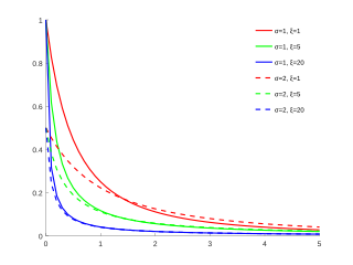
In statistics, the generalized Pareto distribution (GPD) is a family of continuous probability distributions. It is often used to model the tails of another distribution. It is specified by three parameters: location , scale , and shape . Sometimes it is specified by only scale and shape and sometimes only by its shape parameter. Some references give the shape parameter as .
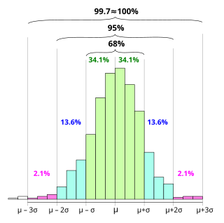
In statistics, the 68–95–99.7 rule, also known as the empirical rule, and sometimes abbreviated 3sr, is a shorthand used to remember the percentage of values that lie within an interval estimate in a normal distribution: approximately 68%, 95%, and 99.7% of the values lie within one, two, and three standard deviations of the mean, respectively.
In probability theory, the multidimensional Chebyshev's inequality is a generalization of Chebyshev's inequality, which puts a bound on the probability of the event that a random variable differs from its expected value by more than a specified amount.
In probability theory, Gauss's inequality gives an upper bound on the probability that a unimodal random variable lies more than any given distance from its mode.
In probability theory, Popoviciu's inequality, named after Tiberiu Popoviciu, is an upper bound on the variance σ2 of any bounded probability distribution. Let M and m be upper and lower bounds on the values of any random variable with a particular probability distribution. Then Popoviciu's inequality states:
In probability theory, concentration inequalities provide mathematical bounds on the probability of a random variable deviating from some value. The deviation or other function of the random variable can be thought of as a secondary random variable. The simplest example of the concentration of such a secondary random variable is the CDF of the first random variable which concentrates the probability to unity. If an analytic form of the CDF is available this provides a concentration equality that provides the exact probability of concentration. It is precisely when the CDF is difficult to calculate or even the exact form of the first random variable is unknown that the applicable concentration inequalities provide useful insight.
For certain applications in linear algebra, it is useful to know properties of the probability distribution of the largest eigenvalue of a finite sum of random matrices. Suppose is a finite sequence of random matrices. Analogous to the well-known Chernoff bound for sums of scalars, a bound on the following is sought for a given parameter t:
In statistics and probability theory, the nonparametric skew is a statistic occasionally used with random variables that take real values. It is a measure of the skewness of a random variable's distribution—that is, the distribution's tendency to "lean" to one side or the other of the mean. Its calculation does not require any knowledge of the form of the underlying distribution—hence the name nonparametric. It has some desirable properties: it is zero for any symmetric distribution; it is unaffected by a scale shift; and it reveals either left- or right-skewness equally well. In some statistical samples it has been shown to be less powerful than the usual measures of skewness in detecting departures of the population from normality.
In probability theory, Cantelli's inequality is an improved version of Chebyshev's inequality for one-sided tail bounds. The inequality states that, for
In probability theory, Eaton's inequality is a bound on the largest values of a linear combination of bounded random variables. This inequality was described in 1974 by Morris L. Eaton.