Decision tree

This article is about decision trees in decision analysis. For the use of the term in machine learning, see Decision tree learning.

Traditionally, decision trees have been created manually.

A decision tree is a decision support recursive partitioning structure that uses a tree-like model of decisions and their possible consequences, including chance event outcomes, resource costs, and utility. It is one way to display an algorithm that only contains conditional control statements.

Decision trees are commonly used in operations research, specifically in decision analysis, ^[1] to help identify a strategy most likely to reach a goal, but are also a popular tool in machine learning.

Overview

A decision tree is a flowchart-like structure in which each internal node represents a "test" on an attribute (e.g. whether a coin flip comes up heads or tails), each branch represents the outcome of the test, and each leaf node represents a class label (decision taken after computing all attributes). The paths from root to leaf represent classification rules.

In decision analysis, a decision tree and the closely related influence diagram are used as a visual and analytical decision support tool, where the expected values (or expected utility) of competing alternatives are calculated.

A decision tree consists of three types of nodes: ^[2]

1. Decision nodes – typically represented by squares
2. Chance nodes – typically represented by circles
3. End nodes – typically represented by triangles

Decision trees are commonly used in operations research and operations management. If, in practice, decisions have to be taken online with no recall under incomplete knowledge, a decision tree should be paralleled by a probability model as a best choice model or online selection model algorithm.^{[ citation needed ]} Another use of decision trees is as a descriptive means for calculating conditional probabilities.

Decision trees, influence diagrams, utility functions, and other decision analysis tools and methods are taught to undergraduate students in schools of business, health economics, and public health, and are examples of operations research or management science methods. These tools are also used to predict decisions of householders in normal and emergency scenarios. ^{[3] [4]}

Decision-tree building blocks

Decision-tree elements

Drawn from left to right, a decision tree has only burst nodes (splitting paths) but no sink nodes (converging paths). So used manually they can grow very big and are then often hard to draw fully by hand. Traditionally, decision trees have been created manually – as the aside example shows – although increasingly, specialized software is employed.

Decision rules

The decision tree can be linearized into decision rules, ^[5] where the outcome is the contents of the leaf node, and the conditions along the path form a conjunction in the if clause. In general, the rules have the form:

if condition1 and condition2 and condition3 then outcome.

Decision rules can be generated by constructing association rules with the target variable on the right. They can also denote temporal or causal relations. ^[6]

Decision tree using flowchart symbols

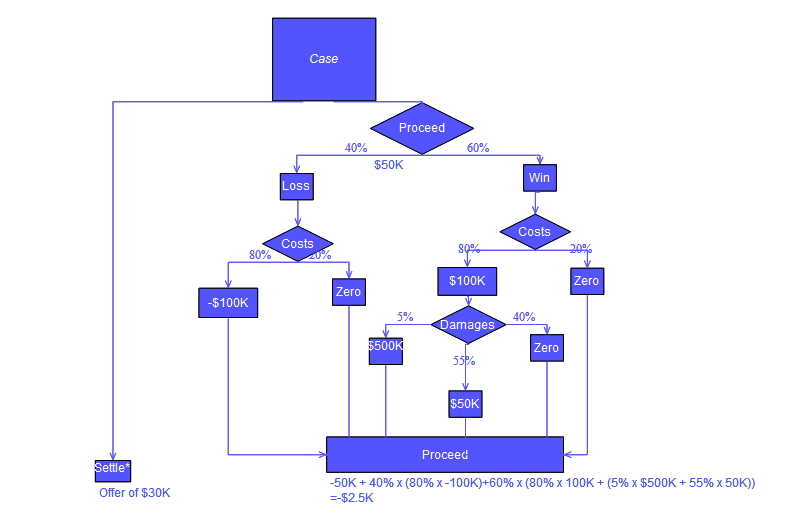
Commonly a decision tree is drawn using flowchart symbols as it is easier for many to read and understand. Note there is a conceptual error in the "Proceed" calculation of the tree shown below; the error relates to the calculation of "costs" awarded in a legal action.

Analysis example

Analysis can take into account the decision maker's (e.g., the company's) preference or utility function, for example:

The basic interpretation in this situation is that the company prefers B's risk and payoffs under realistic risk preference coefficients (greater than $400K—in that range of risk aversion, the company would need to model a third strategy, "Neither A nor B").

Another example, commonly used in operations research courses, is the distribution of lifeguards on beaches (a.k.a. the "Life's a Beach" example). ^[7] The example describes two beaches with lifeguards to be distributed on each beach. There is maximum budget B that can be distributed among the two beaches (in total), and using a marginal returns table, analysts can decide how many lifeguards to allocate to each beach.

Lifeguards on each beach	Drownings prevented in total, beach #1	Drownings prevented in total, beach #2
1	3	1
2	0	4

In this example, a decision tree can be drawn to illustrate the principles of diminishing returns on beach #1.

Beach decision tree

The decision tree illustrates that when sequentially distributing lifeguards, placing a first lifeguard on beach #1 would be optimal if there is only the budget for 1 lifeguard. But if there is a budget for two guards, then placing both on beach #2 would prevent more overall drownings.

Lifeguards

Influence diagram

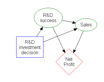
Much of the information in a decision tree can be represented more compactly as an influence diagram, focusing attention on the issues and relationships between events.

The rectangle on the left represents a decision, the ovals represent actions, and the diamond represents results.

Association rule induction

Main article: Decision tree learning

Decision trees can also be seen as generative models of induction rules from empirical data. An optimal decision tree is then defined as a tree that accounts for most of the data, while minimizing the number of levels (or "questions"). ^[8] Several algorithms to generate such optimal trees have been devised, such as ID3/4/5, ^[9] CLS, ASSISTANT, and CART.

Advantages and disadvantages

Among decision support tools, decision trees (and influence diagrams) have several advantages. Decision trees:

• Are simple to understand and interpret. People are able to understand decision tree models after a brief explanation.
• Have value even with little hard data. Important insights can be generated based on experts describing a situation (its alternatives, probabilities, and costs) and their preferences for outcomes.
• Help determine worst, best, and expected values for different scenarios.
• Use a white box model. If a given result is provided by a model.
• Can be combined with other decision techniques.
• The action of more than one decision-maker can be considered.

Disadvantages of decision trees:

• They are unstable, meaning that a small change in the data can lead to a large change in the structure of the optimal decision tree.
• They are often relatively inaccurate. Many other predictors perform better with similar data. This can be remedied by replacing a single decision tree with a random forest of decision trees, but a random forest is not as easy to interpret as a single decision tree.
• For data including categorical variables with different numbers of levels, information gain in decision trees is biased in favor of those attributes with more levels. ^[10]
• Calculations can get very complex, particularly if many values are uncertain and/or if many outcomes are linked.

Optimizing a decision tree

A few things should be considered when improving the accuracy of the decision tree classifier. The following are some possible optimizations to consider when looking to make sure the decision tree model produced makes the correct decision or classification. Note that these things are not the only things to consider but only some.

Increasing the number of levels of the tree

The accuracy of the decision tree can change based on the depth of the decision tree. In many cases, the tree’s leaves are pure nodes. ^[11] When a node is pure, it means that all the data in that node belongs to a single class. ^[12] For example, if the classes in the data set are Cancer and Non-Cancer a leaf node would be considered pure when all the sample data in a leaf node is part of only one class, either cancer or non-cancer. It is important to note that a deeper tree is not always better when optimizing the decision tree. A deeper tree can influence the runtime in a negative way. If a certain classification algorithm is being used, then a deeper tree could mean the runtime of this classification algorithm is significantly slower. There is also the possibility that the actual algorithm building the decision tree will get significantly slower as the tree gets deeper. If the tree-building algorithm being used splits pure nodes, then a decrease in the overall accuracy of the tree classifier could be experienced. Occasionally, going deeper in the tree can cause an accuracy decrease in general, so it is very important to test modifying the depth of the decision tree and selecting the depth that produces the best results. To summarize, observe the points below, we will define the number D as the depth of the tree.

Possible advantages of increasing the number D:

• Accuracy of the decision-tree classification model increases.

Possible disadvantages of increasing D

•  Runtime issues
• Decrease in accuracy in general
• Pure node splits while going deeper can cause issues.

The ability to test the differences in classification results when changing D is imperative. We must be able to easily change and test the variables that could affect the accuracy and reliability of the decision tree-model.

The choice of node-splitting functions

The node splitting function used can have an impact on improving the accuracy of the decision tree. For example, using the information-gain function may yield better results than using the phi function. The phi function is known as a measure of “goodness” of a candidate split at a node in the decision tree. The information gain function is known as a measure of the “reduction in entropy”. In the following, we will build two decision trees. One decision tree will be built using the phi function to split the nodes and one decision tree will be built using the information gain function to split the nodes.

The main advantages and disadvantages of information gain and phi function

• One major drawback of information gain is that the feature that is chosen as the next node in the tree tends to have more unique values. ^[13]
• An advantage of information gain is that it tends to choose the most impactful features that are close to the root of the tree. It is a very good measure for deciding the relevance of some features.
• The phi function is also a good measure for deciding the relevance of some features based on "goodness".

This is the information gain function formula. The formula states the information gain is a function of the entropy of a node of the decision tree minus the entropy of a candidate split at node t of a decision tree.

${\displaystyle I_{\textrm {gain}}(s)=H(t)-H(s,t)}$

This is the phi function formula. The phi function is maximized when the chosen feature splits the samples in a way that produces homogenous splits and have around the same number of samples in each split.

${\displaystyle \Phi (s,t)=(2*P_{L}*P_{R})*Q(s|t)}$

We will set D, which is the depth of the decision tree we are building, to three (D = 3). We also have the following data set of cancer and non-cancer samples and the mutation features that the samples either have or do not have. If a sample has a feature mutation then the sample is positive for that mutation, and it will be represented by one. If a sample does not have a feature mutation then the sample is negative for that mutation, and it will be represented by zero.

To summarize, C stands for cancer and NC stands for non-cancer. The letter M stands for mutation, and if a sample has a particular mutation it will show up in the table as a one and otherwise zero.

The sample data

	M1	M2	M3	M4	M5
C1	0	1	0	1	1
NC1	0	0	0	0	0
NC2	0	0	1	1	0
NC3	0	0	0	0	0
C2	1	1	1	1	1
NC4	0	0	0	1	0

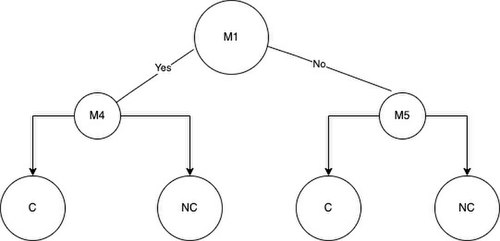
Now, we can use the formulas to calculate the phi function values and information gain values for each M in the dataset. Once all the values are calculated the tree can be produced. The first thing to be done is to select the root node. In information gain and the phi function we consider the optimal split to be the mutation that produces the highest value for information gain or the phi function. Now assume that M1 has the highest phi function value and M4 has the highest information gain value. The M1 mutation will be the root of our phi function tree and M4 will be the root of our information gain tree. You can observe the root nodes below

Figure 1: The left node is the root node of the tree we are building using the phi function to split the nodes. The right node is the root node of the tree we are building using information gain to split the nodes.

Now, once we have chosen the root node we can split the samples into two groups based on whether a sample is positive or negative for the root node mutation. The groups will be called group A and group B. For example, if we use M1 to split the samples in the root node we get NC2 and C2 samples in group A and the rest of the samples NC4, NC3, NC1, C1 in group B.

Disregarding the mutation chosen for the root node, proceed to place the next best features that have the highest values for information gain or the phi function in the left or right child nodes of the decision tree. Once we choose the root node and the two child nodes for the tree of depth = 3 we can just add the leaves. The leaves will represent the final classification decision the model has produced based on the mutations a sample either has or does not have. The left tree is the decision tree we obtain from using information gain to split the nodes and the right tree is what we obtain from using the phi function to split the nodes.

The resulting tree from using information gain to split the nodes

Now assume the classification results from both trees are given using a confusion matrix.

Information gain confusion matrix:

	Predicted: C	Predicted: NC
Actual: C	1	1
Actual: NC	0	4

Phi function confusion matrix:

	Predicted: C	Predicted: NC
Actual: C	2	0
Actual: NC	1	3

The tree using information gain has the same results when using the phi function when calculating the accuracy. When we classify the samples based on the model using information gain we get one true positive, one false positive, zero false negatives, and four true negatives. For the model using the phi function we get two true positives, zero false positives, one false negative, and three true negatives. The next step is to evaluate the effectiveness of the decision tree using some key metrics that will be discussed in the evaluating a decision tree section below. The metrics that will be discussed below can help determine the next steps to be taken when optimizing the decision tree.

Other techniques

The above information is not where it ends for building and optimizing a decision tree. There are many techniques for improving the decision tree classification models we build. One of the techniques is making our decision tree model from a bootstrapped dataset. The bootstrapped dataset helps remove the bias that occurs when building a decision tree model with the same data the model is tested with. The ability to leverage the power of random forests can also help significantly improve the overall accuracy of the model being built. This method generates many decisions from many decision trees and tallies up the votes from each decision tree to make the final classification. There are many techniques, but the main objective is to test building your decision tree model in different ways to make sure it reaches the highest performance level possible.

Evaluating a decision tree

It is important to know the measurements used to evaluate decision trees. The main metrics used are accuracy, sensitivity, specificity, precision, miss rate, false discovery rate, and false omission rate. All these measurements are derived from the number of true positives, false positives, True negatives, and false negatives obtained when running a set of samples through the decision tree classification model. Also, a confusion matrix can be made to display these results. All these main metrics tell something different about the strengths and weaknesses of the classification model built based on your decision tree. For example, a low sensitivity with high specificity could indicate the classification model built from the decision tree does not do well identifying cancer samples over non-cancer samples.

Let us take the confusion matrix below. The confusion matrix shows us the decision tree model classifier built gave 11 true positives, 1 false positive, 45 false negatives, and 105 true negatives.

	Predicted: C	Predicted: NC
Actual: C	11	45
Actual: NC	1	105

We will now calculate the values accuracy, sensitivity, specificity, precision, miss rate, false discovery rate, and false omission rate.

Accuracy:

${\displaystyle Accuracy=(TP+TN)/(TP+TN+FP+FN)}$

${\displaystyle (11+105)\div 162=71.60\%}$

Sensitivity (TPR – true positive rate): ^[14]

${\displaystyle TPR=TP/(TP+FN)}$

${\displaystyle (11)\div (11+45)=19.64\%}$

Specificity (TNR – true negative rate):

${\displaystyle TNR=TN/(TN+FP)}$

${\displaystyle 105\div (105+1)=99.06\%}$

Precision (PPV – positive predictive value):

${\displaystyle PPV=TP/(TP+FP)}$

${\displaystyle 11/(11+1)=91.66\%}$

Miss Rate (FNR – false negative rate):

${\displaystyle FNR=FN/(FN+TP)}$

${\displaystyle 45\div (45+11)=80.35\%}$

False discovery rate (FDR):

${\displaystyle FDR=FP/(FP+TP)}$

${\displaystyle 1\div (1+11)=8.30\%}$

False omission rate (FOR):

${\displaystyle FOR=FN/(FN+TN)}$

${\displaystyle 45\div (45+105)=30.00\%}$

Once we have calculated the key metrics we can make some initial conclusions on the performance of the decision tree model built. The accuracy that we calculated was 71.60%. The accuracy value is good to start but we would like to get our models as accurate as possible while maintaining the overall performance. The sensitivity value of 19.64% means that out of everyone who was actually positive for cancer tested positive. If we look at the specificity value of 99.06% we know that out of all the samples that were negative for cancer actually tested negative. When it comes to sensitivity and specificity it is important to have a balance between the two values, so if we can decrease our specificity to increase the sensitivity that would prove to be beneficial. ^[15] These are just a few examples on how to use these values and the meanings behind them to evaluate the decision tree model and improve upon the next iteration.

See also

• Behavior tree (artificial intelligence, robotics and control)  – Mathematical model of plan execution
• Boosting (machine learning)  – Method in machine learning
• Decision cycle  – Sequence of steps for decision-making
• Decision list
• Decision matrix
• Decision table  – Table specifying actions based on conditions
• Decision tree model  – Model of computational complexity of computation
• Design rationale  – explicit documentation of the reasons behind decisions made when designing a system or artifactPages displaying wikidata descriptions as a fallback
• DRAKON  – Algorithm mapping tool
• Markov chain  – Random process independent of past history
• Random forest  – Tree-based ensemble machine learning method
• Ordinal priority approach  – Multiple-criteria decision analysis method
• Odds algorithm  – Method of computing optimal strategies for last-success problems
• Topological combinatorics
• Truth table  – Mathematical table used in logic

References

1. von Winterfeldt, Detlof; Edwards, Ward (1986). "Decision trees". Decision Analysis and Behavioral Research. Cambridge University Press. pp. 63–89. ISBN   0-521-27304-8.
2. Kamiński, B.; Jakubczyk, M.; Szufel, P. (2017). "A framework for sensitivity analysis of decision trees". Central European Journal of Operations Research. 26 (1): 135–159. doi:10.1007/s10100-017-0479-6. PMC   5767274 . PMID   29375266.
3. Xu, Ningzhe; Lovreglio, Ruggiero; Kuligowski, Erica D.; Cova, Thomas J.; Nilsson, Daniel; Zhao, Xilei (1 March 2023). "Predicting and Assessing Wildfire Evacuation Decision-Making Using Machine Learning: Findings from the 2019 Kincade Fire". Fire Technology. 59 (2): 793–825. doi:10.1007/s10694-023-01363-1. ISSN   1572-8099.
4. Díaz-Ramírez, Jenny; Estrada-García, Juan Alberto; Figueroa-Sayago, Juliana (1 December 2023). "Predicting transport mode choice preferences in a university district with decision tree-based models". City and Environment Interactions. 20: 100118. doi: 10.1016/j.cacint.2023.100118 . ISSN   2590-2520.
5. Quinlan, J. R. (1987). "Simplifying decision trees". International Journal of Man-Machine Studies. 27 (3): 221–234. CiteSeerX   10.1.1.18.4267 . doi:10.1016/S0020-7373(87)80053-6.
6. K. Karimi and H.J. Hamilton (2011), "Generation and Interpretation of Temporal Decision Rules", International Journal of Computer Information Systems and Industrial Management Applications, Volume 3
7. Wagner, Harvey M. (1 September 1975). Principles of Operations Research: With Applications to Managerial Decisions (2nd ed.). Englewood Cliffs, NJ: Prentice Hall. ISBN   9780137095926.
8. R. Quinlan, "Learning efficient classification procedures", Machine Learning: an artificial intelligence approach, Michalski, Carbonell & Mitchell (eds.), Morgan Kaufmann, 1983, p. 463–482. doi : 10.1007/978-3-662-12405-5_15
9. Utgoff, P. E. (1989). Incremental induction of decision trees. Machine learning, 4(2), 161–186. doi : 10.1023/A:1022699900025
10. Deng, H.; Runger, G.; Tuv, E. (2011). Bias of importance measures for multi-valued attributes and solutions. Proceedings of the 21st International Conference on Artificial Neural Networks (ICANN).
11. Larose, Chantal, Daniel (2014). Discovering Knowledge in Data. Hoboken, NJ: John Wiley & Sons. p. 167. ISBN   9780470908747.
12. Plapinger, Thomas (29 July 2017). "What is a Decision Tree?". Towards Data Science. Archived from the original on 10 December 2021. Retrieved 5 December 2021.
13. Tao, Christopher (6 September 2020). "Do Not Use Decision Tree Like Thus". Towards Data Science. Archived from the original on 10 December 2021. Retrieved 10 December 2021.
14. "False Positive Rate | Split Glossary". Split. Retrieved 10 December 2021.
15. "Sensitivity vs Specificity". Analysis & Separations from Technology Networks. Retrieved 10 December 2021.

External links

• Extensive Decision Tree tutorials and examples
• Gallery of example decision trees
• Gradient Boosted Decision Trees