Analysis of variance (ANOVA) is a collection of statistical models and their associated estimation procedures used to analyze the differences among means. ANOVA was developed by the statistician Ronald Fisher. ANOVA is based on the law of total variance, where the observed variance in a particular variable is partitioned into components attributable to different sources of variation. In its simplest form, ANOVA provides a statistical test of whether two or more population means are equal, and therefore generalizes the t-test beyond two means. In other words, the ANOVA is used to test the difference between two or more means.
Multivariate statistics is a subdivision of statistics encompassing the simultaneous observation and analysis of more than one outcome variable, i.e., multivariate random variables. Multivariate statistics concerns understanding the different aims and background of each of the different forms of multivariate analysis, and how they relate to each other. The practical application of multivariate statistics to a particular problem may involve several types of univariate and multivariate analyses in order to understand the relationships between variables and their relevance to the problem being studied.

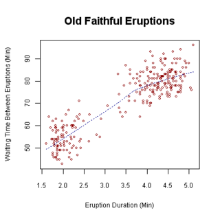
In statistics, correlation or dependence is any statistical relationship, whether causal or not, between two random variables or bivariate data. Although in the broadest sense, "correlation" may indicate any type of association, in statistics it usually refers to the degree to which a pair of variables are linearly related. Familiar examples of dependent phenomena include the correlation between the height of parents and their offspring, and the correlation between the price of a good and the quantity the consumers are willing to purchase, as it is depicted in the so-called demand curve.

In statistics, the Pearson correlation coefficient (PCC) is a correlation coefficient that measures linear correlation between two sets of data. It is the ratio between the covariance of two variables and the product of their standard deviations; thus, it is essentially a normalized measurement of the covariance, such that the result always has a value between −1 and 1. As with covariance itself, the measure can only reflect a linear correlation of variables, and ignores many other types of relationships or correlations. As a simple example, one would expect the age and height of a sample of teenagers from a high school to have a Pearson correlation coefficient significantly greater than 0, but less than 1.
Nonparametric statistics is the type of statistics that is not restricted by assumptions concerning the nature of the population from which a sample is drawn. This is opposed to parametric statistics, for which a problem is restricted a priori by assumptions concerning the specific distribution of the population and parameters. Nonparametric statistics is based on either not assuming a particular distribution or having a distribution specified but with the distribution's parameters not specified in advance. Nonparametric statistics can be used for descriptive statistics or statistical inference. Nonparametric tests are often used when the assumptions of parametric tests are evidently violated.

In statistics, the logistic model is a statistical model that models the probability of an event taking place by having the log-odds for the event be a linear combination of one or more independent variables. In regression analysis, logistic regression is estimating the parameters of a logistic model. Formally, in binary logistic regression there is a single binary dependent variable, coded by an indicator variable, where the two values are labeled "0" and "1", while the independent variables can each be a binary variable or a continuous variable. The corresponding probability of the value labeled "1" can vary between 0 and 1, hence the labeling; the function that converts log-odds to probability is the logistic function, hence the name. The unit of measurement for the log-odds scale is called a logit, from logistic unit, hence the alternative names. See § Background and § Definition for formal mathematics, and § Example for a worked example.
In statistics, a contingency table is a type of table in a matrix format that displays the (multivariate) frequency distribution of the variables. They are heavily used in survey research, business intelligence, engineering, and scientific research. They provide a basic picture of the interrelation between two variables and can help find interactions between them. The term contingency table was first used by Karl Pearson in "On the Theory of Contingency and Its Relation to Association and Normal Correlation", part of the Drapers' Company Research Memoirs Biometric Series I published in 1904.
SUDAAN is a proprietary statistical software package for the analysis of correlated data, including correlated data encountered in complex sample surveys. SUDAAN originated in 1972 at RTI International. Individual commercial licenses are sold for $1,460 a year, or $3,450 permanently.

In statistics, the coefficient of determination, denoted R2 or r2 and pronounced "R squared", is the proportion of the variation in the dependent variable that is predictable from the independent variable(s).
In statistics, resampling is the creation of new samples based on one observed sample. Resampling methods are:
- Permutation tests
- Bootstrapping
- Cross validation
Omnibus tests are a kind of statistical test. They test whether the explained variance in a set of data is significantly greater than the unexplained variance, overall. One example is the F-test in the analysis of variance. There can be legitimate significant effects within a model even if the omnibus test is not significant. For instance, in a model with two independent variables, if only one variable exerts a significant effect on the dependent variable and the other does not, then the omnibus test may be non-significant. This fact does not affect the conclusions that may be drawn from the one significant variable. In order to test effects within an omnibus test, researchers often use contrasts.
In statistics, normality tests are used to determine if a data set is well-modeled by a normal distribution and to compute how likely it is for a random variable underlying the data set to be normally distributed.
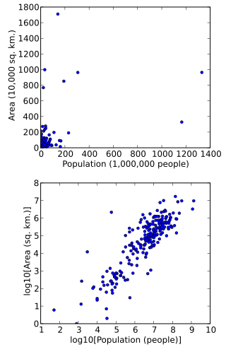
In statistics, data transformation is the application of a deterministic mathematical function to each point in a data set—that is, each data point zi is replaced with the transformed value yi = f(zi), where f is a function. Transforms are usually applied so that the data appear to more closely meet the assumptions of a statistical inference procedure that is to be applied, or to improve the interpretability or appearance of graphs.
The following outline is provided as an overview of and topical guide to regression analysis:
Bivariate analysis is one of the simplest forms of quantitative (statistical) analysis. It involves the analysis of two variables, for the purpose of determining the empirical relationship between them.
WINKS Statistical Data Analytics(SDA) & Graphs is a statistical analysis software package.
Ordinal data is a categorical, statistical data type where the variables have natural, ordered categories and the distances between the categories are not known. These data exist on an ordinal scale, one of four levels of measurement described by S. S. Stevens in 1946. The ordinal scale is distinguished from the nominal scale by having a ranking. It also differs from the interval scale and ratio scale by not having category widths that represent equal increments of the underlying attribute.
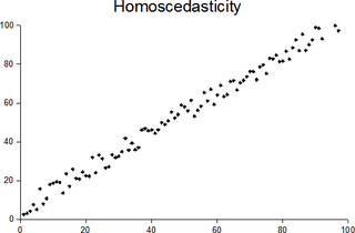
In statistics, a sequence of random variables is homoscedastic if all its random variables have the same finite variance; this is also known as homogeneity of variance. The complementary notion is called heteroscedasticity, also known as heterogeneity of variance. The spellings homoskedasticity and heteroskedasticity are also frequently used. Assuming a variable is homoscedastic when in reality it is heteroscedastic results in unbiased but inefficient point estimates and in biased estimates of standard errors, and may result in overestimating the goodness of fit as measured by the Pearson coefficient.
