
In probability theory and statistics, the negative binomial distribution is a discrete probability distribution that models the number of failures in a sequence of independent and identically distributed Bernoulli trials before a specified (non-random) number of successes occurs. For example, we can define rolling a 6 on some dice as a success, and rolling any other number as a failure, and ask how many failure rolls will occur before we see the third success. In such a case, the probability distribution of the number of failures that appear will be a negative binomial distribution.
In mathematics, random graph is the general term to refer to probability distributions over graphs. Random graphs may be described simply by a probability distribution, or by a random process which generates them. The theory of random graphs lies at the intersection between graph theory and probability theory. From a mathematical perspective, random graphs are used to answer questions about the properties of typical graphs. Its practical applications are found in all areas in which complex networks need to be modeled – many random graph models are thus known, mirroring the diverse types of complex networks encountered in different areas. In a mathematical context, random graph refers almost exclusively to the Erdős–Rényi random graph model. In other contexts, any graph model may be referred to as a random graph.
In statistical mechanics, a canonical ensemble is the statistical ensemble that represents the possible states of a mechanical system in thermal equilibrium with a heat bath at a fixed temperature. The system can exchange energy with the heat bath, so that the states of the system will differ in total energy.
In the study of graphs and networks, the degree of a node in a network is the number of connections it has to other nodes and the degree distribution is the probability distribution of these degrees over the whole network.

In network theory, a giant component is a connected component of a given random graph that contains a significant fraction of the entire graph's vertices.
The Barabási–Albert (BA) model is an algorithm for generating random scale-free networks using a preferential attachment mechanism. Several natural and human-made systems, including the Internet, the World Wide Web, citation networks, and some social networks are thought to be approximately scale-free and certainly contain few nodes with unusually high degree as compared to the other nodes of the network. The BA model tries to explain the existence of such nodes in real networks. The algorithm is named for its inventors Albert-László Barabási and Réka Albert.
Assortativity, or assortative mixing, is a preference for a network's nodes to attach to others that are similar in some way. Though the specific measure of similarity may vary, network theorists often examine assortativity in terms of a node's degree. The addition of this characteristic to network models more closely approximates the behaviors of many real world networks.
In the mathematical field of graph theory, the Erdős–Rényi model refers to one of two closely related models for generating random graphs or the evolution of a random network. These models are named after Hungarian mathematicians Paul Erdős and Alfréd Rényi, who introduced one of the models in 1959. Edgar Gilbert introduced the other model contemporaneously with and independently of Erdős and Rényi. In the model of Erdős and Rényi, all graphs on a fixed vertex set with a fixed number of edges are equally likely. In the model introduced by Gilbert, also called the Erdős–Rényi–Gilbert model, each edge has a fixed probability of being present or absent, independently of the other edges. These models can be used in the probabilistic method to prove the existence of graphs satisfying various properties, or to provide a rigorous definition of what it means for a property to hold for almost all graphs.
The partition function or configuration integral, as used in probability theory, information theory and dynamical systems, is a generalization of the definition of a partition function in statistical mechanics. It is a special case of a normalizing constant in probability theory, for the Boltzmann distribution. The partition function occurs in many problems of probability theory because, in situations where there is a natural symmetry, its associated probability measure, the Gibbs measure, has the Markov property. This means that the partition function occurs not only in physical systems with translation symmetry, but also in such varied settings as neural networks, and applications such as genomics, corpus linguistics and artificial intelligence, which employ Markov networks, and Markov logic networks. The Gibbs measure is also the unique measure that has the property of maximizing the entropy for a fixed expectation value of the energy; this underlies the appearance of the partition function in maximum entropy methods and the algorithms derived therefrom.
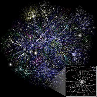
Network science is an academic field which studies complex networks such as telecommunication networks, computer networks, biological networks, cognitive and semantic networks, and social networks, considering distinct elements or actors represented by nodes and the connections between the elements or actors as links. The field draws on theories and methods including graph theory from mathematics, statistical mechanics from physics, data mining and information visualization from computer science, inferential modeling from statistics, and social structure from sociology. The United States National Research Council defines network science as "the study of network representations of physical, biological, and social phenomena leading to predictive models of these phenomena."
Modularity is a measure of the structure of networks or graphs which measures the strength of division of a network into modules. Networks with high modularity have dense connections between the nodes within modules but sparse connections between nodes in different modules. Modularity is often used in optimization methods for detecting community structure in networks. Biological networks, including animal brains, exhibit a high degree of modularity. However, modularity maximization is not statistically consistent, and finds communities in its own null model, i.e. fully random graphs, and therefore it cannot be used to find statistically significant community structures in empirical networks. Furthermore, it has been shown that modularity suffers a resolution limit and, therefore, it is unable to detect small communities.
In statistical mechanics, thermal fluctuations are random deviations of an atomic system from its average state, that occur in a system at equilibrium. All thermal fluctuations become larger and more frequent as the temperature increases, and likewise they decrease as temperature approaches absolute zero.
Evolving networks are dynamic networks that change through time. In each period there are new nodes and edges that join the network while the old ones disappear. Such dynamic behaviour is characteristic for most real-world networks, regardless of their range - global or local. However, networks differ not only in their range but also in their topological structure. It is possible to distinguish:
Robustness, the ability to withstand failures and perturbations, is a critical attribute of many complex systems including complex networks.
Evolution of a random network is a dynamical process in random networks, usually leading to emergence of giant components, accompanied with striking consequences on the network topology.
Lancichinetti–Fortunato–Radicchibenchmark is an algorithm that generates benchmark networks. They have a priori known communities and are used to compare different community detection methods. The advantage of the benchmark over other methods is that it accounts for the heterogeneity in the distributions of node degrees and of community sizes.
Maximal entropy random walk (MERW) is a popular type of biased random walk on a graph, in which transition probabilities are chosen accordingly to the principle of maximum entropy, which says that the probability distribution which best represents the current state of knowledge is the one with largest entropy. While standard random walk chooses for every vertex uniform probability distribution among its outgoing edges, locally maximizing entropy rate, MERW maximizes it globally by assuming uniform probability distribution among all paths in a given graph.
Maximum-entropy random graph models are random graph models used to study complex networks subject to the principle of maximum entropy under a set of structural constraints, which may be global, distributional, or local.
In applied mathematics, the soft configuration model (SCM) is a random graph model subject to the principle of maximum entropy under constraints on the expectation of the degree sequence of sampled graphs. Whereas the configuration model (CM) uniformly samples random graphs of a specific degree sequence, the SCM only retains the specified degree sequence on average over all network realizations; in this sense the SCM has very relaxed constraints relative to those of the CM ("soft" rather than "sharp" constraints). The SCM for graphs of size has a nonzero probability of sampling any graph of size , whereas the CM is restricted to only graphs having precisely the prescribed connectivity structure.
In network science, the activity-driven model is a temporal network model in which each node has a randomly-assigned "activity potential", which governs how it links to other nodes over time.


