Supervised learning (SL) is a paradigm in machine learning where input objects and a desired output value train a model. The training data is processed, building a function that maps new data to expected output values. An optimal scenario will allow for the algorithm to correctly determine output values for unseen instances. This requires the learning algorithm to generalize from the training data to unseen situations in a "reasonable" way. This statistical quality of an algorithm is measured through the so-called generalization error.

In mathematical physics and mathematics, the Pauli matrices are a set of three 2 × 2 complex matrices that are traceless, Hermitian, involutory and unitary. Usually indicated by the Greek letter sigma, they are occasionally denoted by tau when used in connection with isospin symmetries.

The method of least squares is a parameter estimation method in regression analysis based on minimizing the sum of the squares of the residuals made in the results of each individual equation.
In machine learning, early stopping is a form of regularization used to avoid overfitting when training a model with an iterative method, such as gradient descent. Such methods update the model to make it better fit the training data with each iteration. Up to a point, this improves the model's performance on data outside of the training set. Past that point, however, improving the model's fit to the training data comes at the expense of increased generalization error. Early stopping rules provide guidance as to how many iterations can be run before the learner begins to over-fit. Early stopping rules have been employed in many different machine learning methods, with varying amounts of theoretical foundation.

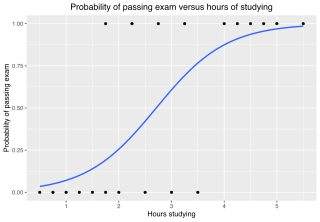
In statistics, the logistic model is a statistical model that models the log-odds of an event as a linear combination of one or more independent variables. In regression analysis, logistic regression estimates the parameters of a logistic model. In binary logistic regression there is a single binary dependent variable, coded by an indicator variable, where the two values are labeled "0" and "1", while the independent variables can each be a binary variable or a continuous variable. The corresponding probability of the value labeled "1" can vary between 0 and 1, hence the labeling; the function that converts log-odds to probability is the logistic function, hence the name. The unit of measurement for the log-odds scale is called a logit, from logistic unit, hence the alternative names. See § Background and § Definition for formal mathematics, and § Example for a worked example.
The information bottleneck method is a technique in information theory introduced by Naftali Tishby, Fernando C. Pereira, and William Bialek. It is designed for finding the best tradeoff between accuracy and complexity (compression) when summarizing a random variable X, given a joint probability distribution p(X,Y) between X and an observed relevant variable Y - and self-described as providing "a surprisingly rich framework for discussing a variety of problems in signal processing and learning".

In applied statistics, total least squares is a type of errors-in-variables regression, a least squares data modeling technique in which observational errors on both dependent and independent variables are taken into account. It is a generalization of Deming regression and also of orthogonal regression, and can be applied to both linear and non-linear models.
Statistical learning theory is a framework for machine learning drawing from the fields of statistics and functional analysis. Statistical learning theory deals with the statistical inference problem of finding a predictive function based on data. Statistical learning theory has led to successful applications in fields such as computer vision, speech recognition, and bioinformatics.
In statistics, multinomial logistic regression is a classification method that generalizes logistic regression to multiclass problems, i.e. with more than two possible discrete outcomes. That is, it is a model that is used to predict the probabilities of the different possible outcomes of a categorically distributed dependent variable, given a set of independent variables.
The normal-inverse Gaussian distribution is a continuous probability distribution that is defined as the normal variance-mean mixture where the mixing density is the inverse Gaussian distribution. The NIG distribution was noted by Blaesild in 1977 as a subclass of the generalised hyperbolic distribution discovered by Ole Barndorff-Nielsen. In the next year Barndorff-Nielsen published the NIG in another paper. It was introduced in the mathematical finance literature in 1997.

In probability theory, Dirichlet processes are a family of stochastic processes whose realizations are probability distributions. In other words, a Dirichlet process is a probability distribution whose range is itself a set of probability distributions. It is often used in Bayesian inference to describe the prior knowledge about the distribution of random variables—how likely it is that the random variables are distributed according to one or another particular distribution.
Monte Carlo in statistical physics refers to the application of the Monte Carlo method to problems in statistical physics, or statistical mechanics.
Non-linear least squares is the form of least squares analysis used to fit a set of m observations with a model that is non-linear in n unknown parameters (m ≥ n). It is used in some forms of nonlinear regression. The basis of the method is to approximate the model by a linear one and to refine the parameters by successive iterations. There are many similarities to linear least squares, but also some significant differences. In economic theory, the non-linear least squares method is applied in (i) the probit regression, (ii) threshold regression, (iii) smooth regression, (iv) logistic link regression, (v) Box–Cox transformed regressors ().
The term generalized logistic distribution is used as the name for several different families of probability distributions. For example, Johnson et al. list four forms, which are listed below.
Stability, also known as algorithmic stability, is a notion in computational learning theory of how a machine learning algorithm output is changed with small perturbations to its inputs. A stable learning algorithm is one for which the prediction does not change much when the training data is modified slightly. For instance, consider a machine learning algorithm that is being trained to recognize handwritten letters of the alphabet, using 1000 examples of handwritten letters and their labels as a training set. One way to modify this training set is to leave out an example, so that only 999 examples of handwritten letters and their labels are available. A stable learning algorithm would produce a similar classifier with both the 1000-element and 999-element training sets.
In computational learning theory, Occam learning is a model of algorithmic learning where the objective of the learner is to output a succinct representation of received training data. This is closely related to probably approximately correct (PAC) learning, where the learner is evaluated on its predictive power of a test set.
In statistics, linear regression is a model that estimates the linear relationship between a scalar response and one or more explanatory variables. A model with exactly one explanatory variable is a simple linear regression; a model with two or more explanatory variables is a multiple linear regression. This term is distinct from multivariate linear regression, which predicts multiple correlated dependent variables rather than a single dependent variable.
In PAC learning, error tolerance refers to the ability of an algorithm to learn when the examples received have been corrupted in some way. In fact, this is a very common and important issue since in many applications it is not possible to access noise-free data. Noise can interfere with the learning process at different levels: the algorithm may receive data that have been occasionally mislabeled, or the inputs may have some false information, or the classification of the examples may have been maliciously adulterated.
An energy-based model (EBM) is an application of canonical ensemble formulation from statistical physics for learning from data. The approach prominently appears in generative artificial intelligence.

The hyperbolastic functions, also known as hyperbolastic growth models, are mathematical functions that are used in medical statistical modeling. These models were originally developed to capture the growth dynamics of multicellular tumor spheres, and were introduced in 2005 by Mohammad Tabatabai, David Williams, and Zoran Bursac. The precision of hyperbolastic functions in modeling real world problems is somewhat due to their flexibility in their point of inflection. These functions can be used in a wide variety of modeling problems such as tumor growth, stem cell proliferation, pharma kinetics, cancer growth, sigmoid activation function in neural networks, and epidemiological disease progression or regression.


![This figure illustrates the relationship between overfitting and the generalization error I[fn] - IS[fn]. Data points were generated from the relationship y = x with white noise added to the y values. In the left column, a set of training points is shown in blue. A seventh order polynomial function was fit to the training data. In the right column, the function is tested on data sampled from the underlying joint probability distribution of x and y. In the top row, the function is fit on a sample dataset of 10 datapoints. In the bottom row, the function is fit on a sample dataset of 100 datapoints. As we can see, for small sample sizes and complex functions, the error on the training set is small but error on the underlying distribution of data is large and we have overfit the data. As a result, generalization error is large. As the number of sample points increases, the prediction error on training and test data converges and generalization error goes to 0. RegressionOverfitting.png](http://upload.wikimedia.org/wikipedia/commons/thumb/c/ca/RegressionOverfitting.png/220px-RegressionOverfitting.png)


