
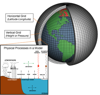
Numerical climate models use quantitative methods to simulate the interactions of the important drivers of climate, including atmosphere, oceans, land surface and ice. They are used for a variety of purposes from study of the dynamics of the climate system to projections of future climate. Climate models may also be qualitative models and also narratives, largely descriptive, of possible futures.
A general circulation model (GCM) is a type of climate model. It employs a mathematical model of the general circulation of a planetary atmosphere or ocean. It uses the Navier–Stokes equations on a rotating sphere with thermodynamic terms for various energy sources. These equations are the basis for computer programs used to simulate the Earth's atmosphere or oceans. Atmospheric and oceanic GCMs are key components along with sea ice and land-surface components.
The oxygen minimum zone (OMZ), sometimes referred to as the shadow zone, is the zone in which oxygen saturation in seawater in the ocean is at its lowest. This zone occurs at depths of about 200 to 1,500 m (660–4,920 ft), depending on local circumstances. OMZs are found worldwide, typically along the western coast of continents, in areas where an interplay of physical and biological processes concurrently lower the oxygen concentration and restrict the water from mixing with surrounding waters, creating a "pool" of water where oxygen concentrations fall from the normal range of 4–6 mg/l to below 2 mg/l.
Numerical weather prediction (NWP) uses mathematical models of the atmosphere and oceans to predict the weather based on current weather conditions. Though first attempted in the 1920s, it was not until the advent of computer simulation in the 1950s that numerical weather predictions produced realistic results. A number of global and regional forecast models are run in different countries worldwide, using current weather observations relayed from radiosondes, weather satellites and other observing systems as inputs.

Sea spray are aerosol particles formed from the ocean, mostly by ejection into Earth's atmosphere by bursting bubbles at the air-sea interface. Sea spray contains both organic matter and inorganic salts that form sea salt aerosol (SSA). SSA has the ability to form cloud condensation nuclei (CCN) and remove anthropogenic aerosol pollutants from the atmosphere. Also, coarse sea spray inhibits lightning.

In fluid dynamics, an eddy is the swirling of a fluid and the reverse current created when the fluid is in a turbulent flow regime. The moving fluid creates a space devoid of downstream-flowing fluid on the downstream side of the object. Fluid behind the obstacle flows into the void creating a swirl of fluid on each edge of the obstacle, followed by a short reverse flow of fluid behind the obstacle flowing upstream, toward the back of the obstacle. This phenomenon is naturally observed behind large emergent rocks in swift-flowing rivers.

An atmospheric model is a mathematical model constructed around the full set of primitive dynamical equations which govern atmospheric motions. It can supplement these equations with parameterizations for turbulent diffusion, radiation, moist processes, heat exchange, soil, vegetation, surface water, the kinematic effects of terrain, and convection. Most atmospheric models are numerical, i.e. they discretize equations of motion. They can predict microscale phenomena such as tornadoes and boundary layer eddies, sub-microscale turbulent flow over buildings, as well as synoptic and global flows. The horizontal domain of a model is either global, covering the entire Earth, or regional (limited-area), covering only part of the Earth. The different types of models run are thermotropic, barotropic, hydrostatic, and nonhydrostatic. Some of the model types make assumptions about the atmosphere which lengthens the time steps used and increases computational speed.

Thin layers are concentrated aggregations of phytoplankton and zooplankton in coastal and offshore waters that are vertically compressed to thicknesses ranging from several centimeters up to a few meters and are horizontally extensive, sometimes for kilometers. Generally, thin layers have three basic criteria: 1) they must be horizontally and temporally persistent; 2) they must not exceed a critical threshold of vertical thickness; and 3) they must exceed a critical threshold of maximum concentration. The precise values for critical thresholds of thin layers has been debated for a long time due to the vast diversity of plankton, instrumentation, and environmental conditions. Thin layers have distinct biological, chemical, optical, and acoustical signatures which are difficult to measure with traditional sampling techniques such as nets and bottles. However, there has been a surge in studies of thin layers within the past two decades due to major advances in technology and instrumentation. Phytoplankton are often measured by optical instruments that can detect fluorescence such as LIDAR, and zooplankton are often measured by acoustic instruments that can detect acoustic backscattering such as ABS. These extraordinary concentrations of plankton have important implications for many aspects of marine ecology, as well as for ocean optics and acoustics. Zooplankton thin layers are often found slightly under phytoplankton layers because many feed on them. Thin layers occur in a wide variety of ocean environments, including estuaries, coastal shelves, fjords, bays, and the open ocean, and they are often associated with some form of vertical structure in the water column, such as pycnoclines, and in zones of reduced flow.
The MEMO model is a Eulerian non-hydrostatic prognostic mesoscale model for wind-flow simulation. It was developed by the Aristotle University of Thessaloniki in collaboration with the Universität Karlsruhe. The MEMO Model together with the photochemical dispersion model MARS are the two core models of the European zooming model (EZM). This model belongs to the family of models designed for describing atmospheric transport phenomena in the local-to-regional scale, frequently referred to as mesoscale air pollution models.
James C. McWilliams is a professor at the UCLA Institute of Geophysics and Planetary Physics and Department of Atmospheric and Oceanic Sciences.
In oceanography, a front is a boundary between two distinct water masses. The formation of fronts depends on multiple physical processes and small differences in these lead to a wide range of front types. They can be as narrow as a few hundreds of metres and as wide as several tens of kilometres. While most fronts form and dissipate relatively quickly, some can persist for long periods of time.
Ocean general circulation models (OGCMs) are a particular kind of general circulation model to describe physical and thermodynamical processes in oceans. The oceanic general circulation is defined as the horizontal space scale and time scale larger than mesoscale. They depict oceans using a three-dimensional grid that include active thermodynamics and hence are most directly applicable to climate studies. They are the most advanced tools currently available for simulating the response of the global ocean system to increasing greenhouse gas concentrations. A hierarchy of OGCMs have been developed that include varying degrees of spatial coverage, resolution, geographical realism, process detail, etc.

A river plume is a freshened water mass that is formed in the sea as a result of mixing of river discharge and saline seawater. River plumes are formed in coastal sea areas at many regions in the World. River plumes generally occupy wide, but shallow sea surface layer bounded by sharp density gradient. The area of a river plume is 3-5 orders of magnitude greater than its depth, therefore, even small rivers with discharge rates ~1–10 m/s form river plumes with horizontal spatial extents ~10–100 m. Areas of river plumes formed by the largest World rivers are ~100–1000 km2. Despite relatively small volume of total freshwater runoff to the World Ocean, river plumes occupy up to 21% of shelf areas of the World Ocean, i.e., several million square kilometers.

The ADCIRC model is a high-performance, cross-platform numerical ocean circulation model popular in simulating storm surge, tides, and coastal circulation problems. Originally developed by Drs. Rick Luettich and Joannes Westerink, the model is developed and maintained by a combination of academic, governmental, and corporate partners, including the University of North Carolina at Chapel Hill, the University of Notre Dame, and the US Army Corps of Engineers. The ADCIRC system includes an independent multi-algorithmic wind forecast model and also has advanced coupling capabilities, allowing it to integrate effects from sediment transport, ice, waves, surface runoff, and baroclinicity.
CICE is a computer model that simulates the growth, melt and movement of sea ice. It has been integrated into many coupled climate system models as well as global ocean and weather forecasting models and is often used as a tool in Arctic and Southern Ocean research. CICE development began in the mid-1990s by the United States Department of Energy (DOE), and it is currently maintained and developed by a group of institutions in North America and Europe known as the CICE Consortium. Its widespread use in earth system science in part owes to the importance of sea ice in determining Earth's planetary albedo, the strength of the global thermohaline circulation in the world's oceans, and in providing surface boundary conditions for atmospheric circulation models, since sea ice occupies a significant proportion (4-6%) of earth's surface. CICE is a type of cryospheric model.
A baroclinic instability is a fluid dynamical instability of fundamental importance in the atmosphere and ocean. It can lead to the formation of transient mesoscale eddies, with a horizontal scale of 10-100 km. In contrast, flows on the largest scale in the ocean are described as ocean currents, the largest scale eddies are mostly created by shearing of two ocean currents and static mesoscale eddies are formed by the flow around an obstacle (as seen in the animation on eddy. Mesoscale eddies are circular currents with swirling motion and account for approximately 90% of the ocean's total kinetic energy. Therefore, they are key in mixing and transport of for example heat, salt and nutrients.
Lisa M. Beal is a professor at the University of Miami known for her work on the Agulhas Current. She is the editor-in-chief of the Journal of Geophysical Research: Oceans.

The North Brazil Current (NBC) retroflects north-eastwards and merges into the North Equatorial Counter Current (NECC). The retroflection occurs in a seasonal pattern when there is strong retroflection from late summer to early winter. There is weakened or no retroflection during other times of the year. Just like in the Agulhas Current, the retroflection also sheds some eddies that make their way to the Caribbean Sea through the Lesser Antilles.
OceanParcels, “Probably A Really Computationally Efficient Lagrangian Simulator”, is a set of python classes and methods that is used to track particles like water, plankton and plastics. It uses the output of Ocean General Circulation Models (OGCM's). OceanParcels main goal is to process the increasingly large amounts of data that is governed by OGCM's. The flow dynamics are simulated using Lagrangian modelling and the geophysical fluid dynamics are simulated with Eulerian modelling or provided through experimental data. OceanParcels is dependent on two principles, namely the ability to read external data sets from different formats and customizable kernels to define particle dynamics.
