Ensemble forecasting

Last updated
Top: Weather Research and Forecasting model simulation of Hurricane Rita tracks. Bottom: The spread of National Hurricane Center multi-model ensemble forecast. WRF rita spread2.jpg
Top: Weather Research and Forecasting model simulation of Hurricane Rita tracks. Bottom: The spread of National Hurricane Center multi-model ensemble forecast.

Ensemble forecasting is a method used in or within numerical weather prediction. Instead of making a single forecast of the most likely weather, a set (or ensemble) of forecasts is produced. This set of forecasts aims to give an indication of the range of possible future states of the atmosphere. Ensemble forecasting is a form of Monte Carlo analysis. The multiple simulations are conducted to account for the two usual sources of uncertainty in forecast models: (1) the errors introduced by the use of imperfect initial conditions, amplified by the chaotic nature of the evolution equations of the atmosphere, which is often referred to as sensitive dependence on initial conditions; and (2) errors introduced because of imperfections in the model formulation, such as the approximate mathematical methods to solve the equations. Ideally, the verified future atmospheric state should fall within the predicted ensemble spread, and the amount of spread should be related to the uncertainty (error) of the forecast. In general, this approach can be used to make probabilistic forecasts of any dynamical system, and not just for weather prediction.

Contents

Instances

Today ensemble predictions are commonly made at most of the major operational weather prediction facilities worldwide, including:

Experimental ensemble forecasts are made at a number of universities, such as the University of Washington, and ensemble forecasts in the US are also generated by the US Navy and Air Force. There are various ways of viewing the data such as spaghetti plots, ensemble means or Postage Stamps where a number of different results from the models run can be compared.

History

As proposed by Edward Lorenz in 1963, it is impossible for long-range forecasts—those made more than two weeks in advance—to predict the state of the atmosphere with any degree of skill owing to the chaotic nature of the fluid dynamics equations involved. [1] Furthermore, existing observation networks have limited spatial and temporal resolution (for example, over large bodies of water such as the Pacific Ocean), which introduces uncertainty into the true initial state of the atmosphere. While a set of equations, known as the Liouville equations, exists to determine the initial uncertainty in the model initialization, the equations are too complex to run in real-time, even with the use of supercomputers. [2] The practical importance of ensemble forecasts derives from the fact that in a chaotic and hence nonlinear system, the rate of growth of forecast error is dependent on starting conditions. An ensemble forecast therefore provides a prior estimate of state-dependent predictability, i.e. an estimate of the types of weather that might occur, given inevitable uncertainties in the forecast initial conditions and in the accuracy of the computational representation of the equations. These uncertainties limit forecast model accuracy to about six days into the future. [3] The first operational ensemble forecasts were produced for sub-seasonal timescales in 1985. [4] However, it was realised that the philosophy underpinning such forecasts was also relevant on shorter timescales – timescales where predictions had previously been made by purely deterministic means.

Edward Epstein recognized in 1969 that the atmosphere could not be completely described with a single forecast run due to inherent uncertainty, and proposed a stochastic dynamic model that produced means and variances for the state of the atmosphere. [5] Although these Monte Carlo simulations showed skill, in 1974 Cecil Leith revealed that they produced adequate forecasts only when the ensemble probability distribution was a representative sample of the probability distribution in the atmosphere. [6] It was not until 1992 that ensemble forecasts began being prepared by the European Centre for Medium-Range Weather Forecasts (ECMWF) and the National Centers for Environmental Prediction (NCEP).

Methods for representing uncertainty

There are two main sources of uncertainty that must be accounted for when making an ensemble weather forecast: initial condition uncertainty and model uncertainty. [7]

Initial condition uncertainty

Initial condition uncertainty arises due to errors in the estimate of the starting conditions for the forecast, both due to limited observations of the atmosphere, and uncertainties involved in using indirect measurements, such as satellite data, to measure the state of atmospheric variables. Initial condition uncertainty is represented by perturbing the starting conditions between the different ensemble members. This explores the range of starting conditions consistent with our knowledge of the current state of the atmosphere, together with its past evolution. There are a number of ways to generate these initial condition perturbations. The ECMWF model, the Ensemble Prediction System (EPS), [8] uses a combination of singular vectors and an ensemble of data assimilations (EDA) to simulate the initial probability density. [9] The singular vector perturbations are more active in the extra-tropics, while the EDA perturbations are more active in the tropics. The NCEP ensemble, the Global Ensemble Forecasting System, uses a technique known as vector breeding. [10] [11]

Model uncertainty

Model uncertainty arises due to the limitations of the forecast model. The process of representing the atmosphere in a computer model involves many simplifications such as the development of parametrisation schemes, which introduce errors into the forecast. Several techniques to represent model uncertainty have been proposed.

Perturbed parameter schemes

When developing a parametrisation scheme, many new parameters are introduced to represent simplified physical processes. These parameters may be very uncertain. For example, the 'entrainment coefficient' represents the turbulent mixing of dry environmental air into a convective cloud, and so represents a complex physical process using a single number. In a perturbed parameter approach, uncertain parameters in the model's parametrisation schemes are identified and their value changed between ensemble members. While in probabilistic climate modelling, such as climateprediction.net, these parameters are often held constant globally and throughout the integration, [12] in modern numerical weather prediction it is more common to stochastically vary the value of the parameters in time and space. [13] The degree of parameter perturbation can be guided using expert judgement, [14] or by directly estimating the degree of parameter uncertainty for a given model. [15]

Stochastic parametrisations

A traditional parametrisation scheme seeks to represent the average effect of the sub grid-scale motion (e.g. convective clouds) on the resolved scale state (e.g. the large scale temperature and wind fields). A stochastic parametrisation scheme recognises that there may be many sub-grid scale states consistent with a particular resolved scale state. Instead of predicting the most likely sub-grid scale motion, a stochastic parametrisation scheme represents one possible realisation of the sub-grid. It does this through including random numbers into the equations of motion. This samples from the probability distribution assigned to uncertain processes. Stochastic parametrisations have significantly improved the skill of weather forecasting models, and are now used in operational forecasting centres worldwide. [16] Stochastic parametrisations were first developed at the European Centre for Medium Range Weather Forecasts. [17]

Multi model ensembles

When many different forecast models are used to try to generate a forecast, the approach is termed multi-model ensemble forecasting. This method of forecasting can improve forecasts when compared to a single model-based approach. [18] When the models within a multi-model ensemble are adjusted for their various biases, this process is known as "superensemble forecasting". This type of a forecast significantly reduces errors in model output. [19] When models of different physical processes are combined, such as combinations of atmospheric, ocean and wave models, the multi-model ensemble is called hyper-ensemble. [20]

Probability assessment

The ensemble forecast is usually evaluated by comparing the ensemble average of the individual forecasts for one forecast variable to the observed value of that variable (the "error"). This is combined with consideration of the degree of agreement between various forecasts within the ensemble system, as represented by their overall standard deviation or "spread". Ensemble spread can be visualised through tools such as spaghetti diagrams, which show the dispersion of one quantity on prognostic charts for specific time steps in the future. Another tool where ensemble spread is used is a meteogram, which shows the dispersion in the forecast of one quantity for one specific location. It is common for the ensemble spread to be too small, such that the observed atmospheric state falls outside of the ensemble forecast. This can lead the forecaster to be overconfident in their forecast. [21] This problem becomes particularly severe for forecasts of the weather about 10 days in advance, [22] particularly if model uncertainty is not accounted for in the forecast.

Reliability and resolution (calibration and sharpness)

The spread of the ensemble forecast indicates how confident the forecaster can be in his or her prediction. When ensemble spread is small and the forecast solutions are consistent within multiple model runs, forecasters perceive more confidence in the forecast in general. [21] When the spread is large, this indicates more uncertainty in the prediction. Ideally, a spread-skill relationship should exist, whereby the spread of the ensemble is a good predictor of the expected error in the ensemble mean. If the forecast is reliable, the observed state will behave as if it is drawn from the forecast probability distribution. Reliability (or calibration) can be evaluated by comparing the standard deviation of the error in the ensemble mean with the forecast spread: for a reliable forecast, the two should match, both at different forecast lead times and for different locations. [23]

The reliability of forecasts of a specific weather event can also be assessed. For example, if 30 of 50 members indicated greater than 1 cm rainfall during the next 24 h, the probability of exceeding 1 cm could be estimated to be 60%. The forecast would be considered reliable if, considering all the situations in the past when a 60% probability was forecast, on 60% of those occasions did the rainfall actually exceed 1 cm. In practice, the probabilities generated from operational weather ensemble forecasts are not highly reliable, though with a set of past forecasts (reforecasts or hindcasts) and observations, the probability estimates from the ensemble can be adjusted to ensure greater reliability.

Another desirable property of ensemble forecasts is resolution. This is an indication of how much the forecast deviates from the climatological event frequency – provided that the ensemble is reliable, increasing this deviation will increase the usefulness of the forecast. This forecast quality can also be considered in terms of sharpness, or how small the spread of the forecast is. The key aim of a forecaster should be to maximise sharpness, while maintaining reliability. [24] Forecasts at long leads will inevitably not be particularly sharp (have particularly high resolution), for the inevitable (albeit usually small) errors in the initial condition will grow with increasing forecast lead until the expected difference between two model states is as large as the difference between two random states from the forecast model's climatology.

Calibration of ensemble forecasts

If ensemble forecasts are to be used for predicting probabilities of observed weather variables they typically need calibration in order to create unbiased and reliable forecasts. For forecasts of temperature one simple and effective method of calibration is linear regression, often known in this context as model output statistics. The linear regression model takes the ensemble mean as a predictor for the real temperature, ignores the distribution of ensemble members around the mean, and predicts probabilities using the distribution of residuals from the regression. In this calibration setup the value of the ensemble in improving the forecast is then that the ensemble mean typically gives a better forecast than any single ensemble member would, and not because of any information contained in the width or shape of the distribution of the members in the ensemble around the mean. However, in 2004, a generalisation of linear regression (now known as Nonhomogeneous Gaussian regression) was introduced [25] that uses a linear transformation of the ensemble spread to give the width of the predictive distribution, and it was shown that this can lead to forecasts with higher skill than those based on linear regression alone. This proved for the first time that information in the shape of the distribution of the members of an ensemble around the mean, in this case summarized by the ensemble spread, can be used to improve forecasts relative to linear regression. Whether or not linear regression can be beaten by using the ensemble spread in this way varies, depending on the forecast system, forecast variable and lead time.

Predicting the size of forecast changes

In addition to being used to improve predictions of uncertainty, the ensemble spread can also be used as a predictor for the likely size of changes in the mean forecast from one forecast to the next. [26] This works because, in some ensemble forecast systems, narrow ensembles tend to precede small changes in the mean, while wide ensembles tend to precede larger changes in the mean. This has applications in the trading industries, for whom understanding the likely sizes of future forecast changes can be important.

Co-ordinated research

The Observing System Research and Predictability Experiment (THORPEX) is a 10-year international research and development programme to accelerate improvements in the accuracy of one-day to two-week high impact weather forecasts for the benefit of society, the economy and the environment. It establishes an organizational framework that addresses weather research and forecast problems whose solutions will be accelerated through international collaboration among academic institutions, operational forecast centres and users of forecast products.

One of its key components is THORPEX Interactive Grand Global Ensemble (TIGGE), a World Weather Research Programme to accelerate the improvements in the accuracy of 1-day to 2 week high-impact weather forecasts for the benefit of humanity. Centralized archives of ensemble model forecast data, from many international centers, are used to enable extensive data sharing and research.

See also

Related Research Articles

<span class="mw-page-title-main">European Centre for Medium-Range Weather Forecasts</span> European intergovernmental weather computation organisation based in the UK

The European Centre for Medium-Range Weather Forecasts (ECMWF) is an independent intergovernmental organisation supported by most of the nations of Europe. It is based at three sites: Shinfield Park, Reading, United Kingdom; Bologna, Italy; and Bonn, Germany. It operates one of the largest supercomputer complexes in Europe and the world's largest archive of numerical weather prediction data.

<span class="mw-page-title-main">Weather forecasting</span> Science and technology application

Weather forecasting is the application of science and technology to predict the conditions of the atmosphere for a given location and time. People have attempted to predict the weather informally for millennia and formally since the 19th century.

<span class="mw-page-title-main">General circulation model</span> Type of climate model

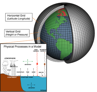
A general circulation model (GCM) is a type of climate model. It employs a mathematical model of the general circulation of a planetary atmosphere or ocean. It uses the Navier–Stokes equations on a rotating sphere with thermodynamic terms for various energy sources. These equations are the basis for computer programs used to simulate the Earth's atmosphere or oceans. Atmospheric and oceanic GCMs are key components along with sea ice and land-surface components.

<span class="mw-page-title-main">Numerical weather prediction</span> Weather prediction using mathematical models of the atmosphere and oceans

Numerical weather prediction (NWP) uses mathematical models of the atmosphere and oceans to predict the weather based on current weather conditions. Though first attempted in the 1920s, it was not until the advent of computer simulation in the 1950s that numerical weather predictions produced realistic results. A number of global and regional forecast models are run in different countries worldwide, using current weather observations relayed from radiosondes, weather satellites and other observing systems as inputs.

Data assimilation is a mathematical discipline that seeks to optimally combine theory with observations. There may be a number of different goals sought – for example, to determine the optimal state estimate of a system, to determine initial conditions for a numerical forecast model, to interpolate sparse observation data using knowledge of the system being observed, to set numerical parameters based on training a model from observed data. Depending on the goal, different solution methods may be used. Data assimilation is distinguished from other forms of machine learning, image analysis, and statistical methods in that it utilizes a dynamical model of the system being analyzed.

The Brier Score is a strictly proper score function or strictly proper scoring rule that measures the accuracy of probabilistic predictions. For unidimensional predictions, it is strictly equivalent to the mean squared error as applied to predicted probabilities.
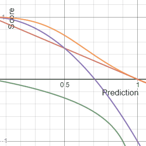
Probabilistic forecasting summarizes what is known about, or opinions about, future events. In contrast to single-valued forecasts, probabilistic forecasts assign a probability to each of a number of different outcomes, and the complete set of probabilities represents a probability forecast. Thus, probabilistic forecasting is a type of probabilistic classification.

<span class="mw-page-title-main">Tropical cyclone forecast model</span> Computer program that uses meteorological data to forecast tropical cyclones

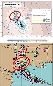
A tropical cyclone forecast model is a computer program that uses meteorological data to forecast aspects of the future state of tropical cyclones. There are three types of models: statistical, dynamical, or combined statistical-dynamic. Dynamical models utilize powerful supercomputers with sophisticated mathematical modeling software and meteorological data to calculate future weather conditions. Statistical models forecast the evolution of a tropical cyclone in a simpler manner, by extrapolating from historical datasets, and thus can be run quickly on platforms such as personal computers. Statistical-dynamical models use aspects of both types of forecasting. Four primary types of forecasts exist for tropical cyclones: track, intensity, storm surge, and rainfall. Dynamical models were not developed until the 1970s and the 1980s, with earlier efforts focused on the storm surge problem.

<span class="mw-page-title-main">Atmospheric model</span> Mathematical model of atmospheric motions

In atmospheric science, an atmospheric model is a mathematical model constructed around the full set of primitive, dynamical equations which govern atmospheric motions. It can supplement these equations with parameterizations for turbulent diffusion, radiation, moist processes, heat exchange, soil, vegetation, surface water, the kinematic effects of terrain, and convection. Most atmospheric models are numerical, i.e. they discretize equations of motion. They can predict microscale phenomena such as tornadoes and boundary layer eddies, sub-microscale turbulent flow over buildings, as well as synoptic and global flows. The horizontal domain of a model is either global, covering the entire Earth, or regional (limited-area), covering only part of the Earth. The different types of models run are thermotropic, barotropic, hydrostatic, and nonhydrostatic. Some of the model types make assumptions about the atmosphere which lengthens the time steps used and increases computational speed.

In weather forecasting, model output statistics (MOS) is a multiple linear regression technique in which predictands, often near-surface quantities, are related statistically to one or more predictors. The predictors are typically forecasts from a numerical weather prediction (NWP) model, climatic data, and, if applicable, recent surface observations. Thus, output from NWP models can be transformed by the MOS technique into sensible weather parameters that are familiar to a layperson.

<span class="mw-page-title-main">Quantitative precipitation forecast</span> Expected amount of melted precipitation

The quantitative precipitation forecast is the expected amount of melted precipitation accumulated over a specified time period over a specified area. A QPF will be created when precipitation amounts reaching a minimum threshold are expected during the forecast's valid period. Valid periods of precipitation forecasts are normally synoptic hours such as 00:00, 06:00, 12:00 and 18:00 GMT. Terrain is considered in QPFs by use of topography or based upon climatological precipitation patterns from observations with fine detail. Starting in the mid-to-late 1990s, QPFs were used within hydrologic forecast models to simulate impact to rivers throughout the United States. Forecast models show significant sensitivity to humidity levels within the planetary boundary layer, or in the lowest levels of the atmosphere, which decreases with height. QPF can be generated on a quantitative, forecasting amounts, or a qualitative, forecasting the probability of a specific amount, basis. Radar imagery forecasting techniques show higher skill than model forecasts within 6 to 7 hours of the time of the radar image. The forecasts can be verified through use of rain gauge measurements, weather radar estimates, or a combination of both. Various skill scores can be determined to measure the value of the rainfall forecast.

<span class="mw-page-title-main">History of numerical weather prediction</span> Aspect of meteorological history

The history of numerical weather prediction considers how current weather conditions as input into mathematical models of the atmosphere and oceans to predict the weather and future sea state has changed over the years. Though first attempted manually in the 1920s, it was not until the advent of the computer and computer simulation that computation time was reduced to less than the forecast period itself. ENIAC was used to create the first forecasts via computer in 1950, and over the years more powerful computers have been used to increase the size of initial datasets and use more complicated versions of the equations of motion. The development of global forecasting models led to the first climate models. The development of limited area (regional) models facilitated advances in forecasting the tracks of tropical cyclone as well as air quality in the 1970s and 1980s.

A prognostic chart is a map displaying the likely weather forecast for a future time. Such charts generated by atmospheric models as output from numerical weather prediction and contain a variety of information such as temperature, wind, precipitation and weather fronts. They can also indicate derived atmospheric fields such as vorticity, stability indices, or frontogenesis. Forecast errors need to be taken into account and can be determined either via absolute error, or by considering persistence and absolute error combined.

Edward Epstein was an American meteorologist who pioneered the use of statistical methods in weather forecasting and the development of ensemble forecasting techniques.

<span class="mw-page-title-main">Tim Palmer (physicist)</span> British meteorologist

Timothy Noel Palmer CBE FRS is a mathematical physicist by training. He has spent most of his career working on the dynamics and predictability of weather and climate. Among various research achievements, he pioneered the development of probabilistic ensemble forecasting techniques for weather and climate prediction. These techniques are now standard in operational weather and climate prediction around the world, and are central for reliable decision making for many commercial and humanitarian applications.

The THORPEX Interactive Grand Global Ensemble (TIGGE) is an implementation of ensemble forecasting for global weather forecasting and is part of THORPEX, an international research programme established in 2003 by the World Meteorological Organization to accelerate improvements in the utility and accuracy of weather forecasts up to two weeks ahead.

The North American Ensemble Forecast System (NAEFS) is a joint project involving the Meteorological Service of Canada (MSC) in Canada, the National Weather Service (NWS) in the United States, and the National Meteorological Service of Mexico (NMSM) in Mexico providing numerical weather prediction ensemble guidance for the 1- to 16-day forecast period. The NAEFS combines the Canadian MSC and the US NWS global ensemble prediction systems, improving probabilistic operational guidance over what can be built from any individual country's ensemble. Model guidance from the NAEFS is incorporated into the forecasts of the respective national agencies.

The cost-loss model, also called the cost/loss model or the cost-loss decision model, is a model used to understand how the predicted probability of adverse events affects the decision of whether to take a costly precautionary measure to protect oneself against losses from that event. The threshold probability above which it makes sense to take the precautionary measure equals the ratio of the cost of the preventative measure to the loss averted, and this threshold is termed the cost/loss ratio or cost-loss ratio. The model is typically used in the context of using prediction about weather conditions to decide whether to take a precautionary measure or not.

Non-homogeneous Gaussian regression (NGR) is a type of statistical regression analysis used in the atmospheric sciences as a way to convert ensemble forecasts into probabilistic forecasts. Relative to simple linear regression, NGR uses the ensemble spread as an additional predictor, which is used to improve the prediction of uncertainty and allows the predicted uncertainty to vary from case to case. The prediction of uncertainty in NGR is derived from both past forecast errors statistics and the ensemble spread. NGR was originally developed for site-specific medium range temperature forecasting, but has since also been applied to site-specific medium-range wind forecasting and to seasonal forecasts, and has been adapted for precipitation forecasting. The introduction of NGR was the first demonstration that probabilistic forecasts that take account of the varying ensemble spread could achieve better skill scores than forecasts based on standard Model output statistics approaches applied to the ensemble mean.

References

  1. Cox, John D. (2002). Storm Watchers . John Wiley & Sons, Inc. pp.  222–224. ISBN   978-0-471-38108-2.
  2. Manousos, Peter (2006-07-19). "Ensemble Prediction Systems". Hydrometeorological Prediction Center . Retrieved 2010-12-31.
  3. Weickmann, Klaus, Jeff Whitaker, Andres Roubicek and Catherine Smith (2001-12-01). The Use of Ensemble Forecasts to Produce Improved Medium Range (3–15 days) Weather Forecasts. Climate Diagnostics Center. Retrieved 2007-02-16.
  4. Palmer, Tim (2018). "The ECMWF ensemble prediction system: Looking back (more than) 25 years and projecting forward 25 years". Quarterly Journal of the Royal Meteorological Society. 145 (S1): 12–24. arXiv: 1803.06940 . Bibcode:2019QJRMS.145S..12P. doi:10.1002/qj.3383. ISSN   1477-870X. S2CID   4944687.
  5. Epstein, E.S. (December 1969). "Stochastic dynamic prediction". Tellus A . 21 (6): 739–759. Bibcode:1969Tell...21..739E. doi:10.1111/j.2153-3490.1969.tb00483.x.
  6. Leith, C.E. (June 1974). "Theoretical Skill of Monte Carlo Forecasts". Monthly Weather Review . 102 (6): 409–418. Bibcode:1974MWRv..102..409L. doi: 10.1175/1520-0493(1974)102<0409:TSOMCF>2.0.CO;2 . ISSN   1520-0493.
  7. Slingo, Julia; Palmer, Tim (2011-12-13). "Uncertainty in weather and climate prediction". Phil. Trans. R. Soc. A. 369 (1956): 4751–4767. Bibcode:2011RSPTA.369.4751S. doi:10.1098/rsta.2011.0161. ISSN   1364-503X. PMC   3270390 . PMID   22042896.
  8. "The Ensemble Prediction System (EPS)". ECMWF. Archived from the original on 2010-10-30. Retrieved 2011-01-05.
  9. "Quantifying forecast uncertainty | ECMWF". www.ecmwf.int. 2013-11-29. Retrieved 2016-11-20.
  10. Toth, Zoltan; Kalnay, Eugenia (December 1997). "Ensemble Forecasting at NCEP and the Breeding Method". Monthly Weather Review . 125 (12): 3297–3319. Bibcode:1997MWRv..125.3297T. CiteSeerX   10.1.1.324.3941 . doi:10.1175/1520-0493(1997)125<3297:EFANAT>2.0.CO;2. ISSN   1520-0493. S2CID   14668576.
  11. Molteni, F.; Buizza, R.; Palmer, T.N.; Petroliagis, T. (January 1996). "The ECMWF Ensemble Prediction System: Methodology and validation". Quarterly Journal of the Royal Meteorological Society. 122 (529): 73–119. Bibcode:1996QJRMS.122...73M. doi:10.1002/qj.49712252905.
  12. "Perturbed Physics Ensembles | climateprediction.net". www.climateprediction.net. Retrieved 2016-11-20.
  13. McCabe, Anne; Swinbank, Richard; Tennant, Warren; Lock, Adrian (2016-10-01). "Representing model uncertainty in the Met Office convection-permitting ensemble prediction system and its impact on fog forecasting". Quarterly Journal of the Royal Meteorological Society. 142 (700): 2897–2910. Bibcode:2016QJRMS.142.2897M. doi:10.1002/qj.2876. ISSN   1477-870X. S2CID   124729470.
  14. Ollinaho, Pirkka; Lock, Sarah-Jane; Leutbecher, Martin; Bechtold, Peter; Beljaars, Anton; Bozzo, Alessio; Forbes, Richard M.; Haiden, Thomas; Hogan, Robin J. (2016-10-01). "Towards process-level representation of model uncertainties: Stochastically perturbed parametrisations in the ECMWF ensemble". Quarterly Journal of the Royal Meteorological Society. 143 (702): 408–422. Bibcode:2017QJRMS.143..408O. doi:10.1002/qj.2931. ISSN   1477-870X. S2CID   125248441.
  15. Christensen, H. M.; Moroz, I. M.; Palmer, T. N. (2015-02-04). "Stochastic and Perturbed Parameter Representations of Model Uncertainty in Convection Parameterization". Journal of the Atmospheric Sciences. 72 (6): 2525–2544. Bibcode:2015JAtS...72.2525C. doi:10.1175/JAS-D-14-0250.1. ISSN   0022-4928. S2CID   123117331.
  16. Berner, Judith; Achatz, Ulrich; Batté, Lauriane; Bengtsson, Lisa; De La Cámara, Alvaro; Christensen, Hannah M.; Colangeli, Matteo; Coleman, Danielle R. B.; Crommelin, Daan (2016-07-19). "Stochastic Parameterization: Towards a new view of Weather and Climate Models". Bulletin of the American Meteorological Society. 98 (3): 565. arXiv: 1510.08682 . Bibcode:2017BAMS...98..565B. doi:10.1175/BAMS-D-15-00268.1. ISSN   0003-0007. S2CID   33134061.
  17. Buizza, R.; Milleer, M.; Palmer, T. N. (1999-10-01). "Stochastic representation of model uncertainties in the ECMWF ensemble prediction system". Quarterly Journal of the Royal Meteorological Society. 125 (560): 2887–2908. Bibcode:1999QJRMS.125.2887B. doi:10.1002/qj.49712556006. ISSN   1477-870X. S2CID   123346799.
  18. Zhou, Binbin and Jun Du (February 2010). "Fog Prediction From a Multimodel Mesoscale Ensemble Prediction System" (PDF). Weather and Forecasting . 25 (1): 303. Bibcode:2010WtFor..25..303Z. doi:10.1175/2009WAF2222289.1. S2CID   4947206 . Retrieved 2011-01-02.
  19. Cane, D. and M. Milelli (2010-02-12). "Multimodel SuperEnsemble technique for quantitative precipitation forecasts in Piemonte region". Natural Hazards and Earth System Sciences. 10 (2): 265. Bibcode:2010NHESS..10..265C. doi: 10.5194/nhess-10-265-2010 .
  20. Vandenbulcke, L.; et al. (2009). "Super-Ensemble techniques: application to surface drift prediction" (PDF). Progress in Oceanography. 82 (3): 149–167. Bibcode:2009PrOce..82..149V. doi:10.1016/j.pocean.2009.06.002.
  21. 1 2 Warner, Thomas Tomkins (2010). Numerical Weather and Climate Prediction. Cambridge University Press. pp. 266–275. ISBN   978-0-521-51389-0.
  22. Palmer, T.N.; G.J. Shutts; R. Hagedorn; F.J. Doblas-Reyes; T. Jung; M. Leutbecher (May 2005). "Representing Model Uncertainty in Weather and Climate Prediction". Annual Review of Earth and Planetary Sciences . 33: 163–193. Bibcode:2005AREPS..33..163P. doi:10.1146/annurev.earth.33.092203.122552.
  23. Leutbecher, M.; Palmer, T. N. (2008-03-20). "Ensemble forecasting". Journal of Computational Physics. Predicting weather, climate and extreme events. 227 (7): 3515–3539. Bibcode:2008JCoPh.227.3515L. doi:10.1016/j.jcp.2007.02.014.
  24. Gneiting, Tilmann; Balabdaoui, Fadoua; Raftery, Adrian E. (2007-04-01). "Probabilistic forecasts, calibration and sharpness". Journal of the Royal Statistical Society, Series B. 69 (2): 243–268. CiteSeerX   10.1.1.142.9002 . doi:10.1111/j.1467-9868.2007.00587.x. S2CID   123181502.
  25. Jewson, S; Brix, A; Ziehmann, C (2004). "A new parametric model for the assessment and calibration of medium‐range ensemble temperature forecasts". Atmospheric Science Letters. 5 (5): 96–102. arXiv: physics/0308057 . Bibcode:2004AtScL...5...96J. doi:10.1002/asl.69. S2CID   118358858.
  26. Jewson, S; Ziehmann, C (2004). "Using ensemble forecasts to predict the size of forecast changes, with application to weather swap value at risk". Atmospheric Science Letters. 4 (1–4): 15–27. doi: 10.1016/S1530-261X(03)00003-3 .

Further reading