String vibration

Vibration, standing waves in a string. The fundamental and the first 5 overtones in the harmonic series.

A vibration in a string is a wave. Resonance causes a vibrating string to produce a sound with constant frequency, i.e. constant pitch. If the length or tension of the string is correctly adjusted, the sound produced is a musical tone. Vibrating strings are the basis of string instruments such as guitars, cellos, and pianos.

Wave

The velocity of propagation of a wave in a string (${\displaystyle v}$) is proportional to the square root of the force of tension of the string (${\displaystyle T}$) and inversely proportional to the square root of the linear density (${\displaystyle \mu }$) of the string:

${\displaystyle v={\sqrt {T \over \mu }}.}$

This relationship was discovered by Vincenzo Galilei in the late 1500s. ^{[ citation needed ]}

Derivation

Illustration for a vibrating string

Source: ^[1]

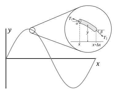
Let ${\displaystyle \Delta x}$ be the length of a piece of string, ${\displaystyle m}$ its mass, and ${\displaystyle \mu }$ its linear density. If angles ${\displaystyle \alpha }$ and ${\displaystyle \beta }$ are small, then the horizontal components of tension on either side can both be approximated by a constant ${\displaystyle T}$, for which the net horizontal force is zero. Accordingly, using the small angle approximation, the horizontal tensions acting on both sides of the string segment are given by

${\displaystyle T_{1x}=T_{1}\cos(\alpha )\approx T.}$

${\displaystyle T_{2x}=T_{2}\cos(\beta )\approx T.}$

From Newton's second law for the vertical component, the mass (which is the product of its linear density and length) of this piece times its acceleration, ${\displaystyle a}$, will be equal to the net force on the piece:

${\displaystyle \Sigma F_{y}=T_{1y}-T_{2y}=-T_{2}\sin(\beta )+T_{1}\sin(\alpha )=\Delta ma\approx \mu \Delta x{\frac {\partial ^{2}y}{\partial t^{2}}}.}$

Dividing this expression by ${\displaystyle T}$ and substituting the first and second equations obtains (we can choose either the first or the second equation for ${\displaystyle T}$, so we conveniently choose each one with the matching angle ${\displaystyle \beta }$ and ${\displaystyle \alpha }$)

${\displaystyle -{\frac {T_{2}\sin(\beta )}{T_{2}\cos(\beta )}}+{\frac {T_{1}\sin(\alpha )}{T_{1}\cos(\alpha )}}=-\tan(\beta )+\tan(\alpha )={\frac {\mu \Delta x}{T}}{\frac {\partial ^{2}y}{\partial t^{2}}}.}$

According to the small-angle approximation, the tangents of the angles at the ends of the string piece are equal to the slopes at the ends, with an additional minus sign due to the definition of ${\displaystyle \alpha }$ and ${\displaystyle \beta }$. Using this fact and rearranging provides

${\displaystyle {\frac {1}{\Delta x}}\left(\left.{\frac {\partial y}{\partial x}}\right|^{x+\Delta x}-\left.{\frac {\partial y}{\partial x}}\right|^{x}\right)={\frac {\mu }{T}}{\frac {\partial ^{2}y}{\partial t^{2}}}.}$

In the limit that ${\displaystyle \Delta x}$ approaches zero, the left hand side is the definition of the second derivative of ${\displaystyle y}$:

${\displaystyle {\frac {\partial ^{2}y}{\partial x^{2}}}={\frac {\mu }{T}}{\frac {\partial ^{2}y}{\partial t^{2}}}.}$

This is the wave equation for ${\displaystyle y(x,t)}$, and the coefficient of the second time derivative term is equal to ${\displaystyle {\frac {1}{v^{2}}}}$; thus

${\displaystyle v={\sqrt {T \over \mu }},}$

Where ${\displaystyle v}$ is the speed of propagation of the wave in the string (see the article on the wave equation for more about this). However, this derivation is only valid for small amplitude vibrations; for those of large amplitude, ${\displaystyle \Delta x}$ is not a good approximation for the length of the string piece, the horizontal component of tension is not necessarily constant. The horizontal tensions are not well approximated by ${\displaystyle T}$.

Frequency of the wave

Once the speed of propagation is known, the frequency of the sound produced by the string can be calculated. The speed of propagation of a wave is equal to the wavelength ${\displaystyle \lambda }$ divided by the period ${\displaystyle \tau }$, or multiplied by the frequency ${\displaystyle f}$:

${\displaystyle v={\frac {\lambda }{\tau }}=\lambda f.}$

If the length of the string is ${\displaystyle L}$, the fundamental harmonic is the one produced by the vibration whose nodes are the two ends of the string, so ${\displaystyle L}$ is half of the wavelength of the fundamental harmonic. Hence one obtains Mersenne's laws:

${\displaystyle f={\frac {v}{2L}}={1 \over 2L}{\sqrt {T \over \mu }}}$

where ${\displaystyle T}$ is the tension (in Newtons), ${\displaystyle \mu }$ is the linear density (that is, the mass per unit length), and ${\displaystyle L}$ is the length of the vibrating part of the string. Therefore:

• the shorter the string, the higher the frequency of the fundamental
• the higher the tension, the higher the frequency of the fundamental
• the lighter the string, the higher the frequency of the fundamental

Moreover, if we take the nth harmonic as having a wavelength given by ${\displaystyle \lambda _{n}=2L/n}$, then we easily get an expression for the frequency of the nth harmonic:

${\displaystyle f_{n}={\frac {nv}{2L}}}$

And for a string under a tension T with linear density ${\displaystyle \mu }$, then

${\displaystyle f_{n}={\frac {n}{2L}}{\sqrt {\frac {T}{\mu }}}}$

Observing string vibrations

One can see the waveforms on a vibrating string if the frequency is low enough and the vibrating string is held in front of a CRT screen such as one of a television or a computer (not of an analog oscilloscope). This effect is called the stroboscopic effect, and the rate at which the string seems to vibrate is the difference between the frequency of the string and the refresh rate of the screen. The same can happen with a fluorescent lamp, at a rate that is the difference between the frequency of the string and the frequency of the alternating current. (If the refresh rate of the screen equals the frequency of the string or an integer multiple thereof, the string will appear still but deformed.) In daylight and other non-oscillating light sources, this effect does not occur and the string appears still but thicker, and lighter or blurred, due to persistence of vision.

A similar but more controllable effect can be obtained using a stroboscope. This device allows matching the frequency of the xenon flash lamp to the frequency of vibration of the string. In a dark room, this clearly shows the waveform. Otherwise, one can use bending or, perhaps more easily, by adjusting the machine heads, to obtain the same, or a multiple, of the AC frequency to achieve the same effect. For example, in the case of a guitar, the 6th (lowest pitched) string pressed to the third fret gives a G at 97.999 Hz. A slight adjustment can alter it to 100 Hz, exactly one octave above the alternating current frequency in Europe and most countries in Africa and Asia, 50 Hz. In most countries of the Americas—where the AC frequency is 60 Hz—altering A# on the fifth string, first fret from 116.54 Hz to 120 Hz produces a similar effect.

Real-world example

See also: Guitar tunings, 12 equal temperament, and A440 (pitch standard)

A Wikipedia user's Jackson Professional Soloist XL electric guitar has a nut-to-bridge distance (corresponding to ${\displaystyle L}$ above) of 255⁄8 in. and D'Addario XL Nickel-wound Super-light-gauge EXL-120 electric guitar strings with the following manufacturer specs:

D'Addario EXL-120 manufacturer specs

String no.	Thickness [in.] (${\displaystyle d}$)	Recommended tension [lbs.] (${\displaystyle T}$)	${\displaystyle \rho }$ [g/cm3]
1	0.00899	13.1	7.726 (steel alloy)
2	0.0110	11.0	"
3	0.0160	14.7	"
4	0.0241	15.8	6.533 (nickel-wound steel alloy)
5	0.0322	15.8	"
6	0.0416	14.8	"

Given the above specs, what would the computed vibrational frequencies (${\displaystyle f}$) of the above strings' fundamental harmonics be if the strings were strung at the tensions recommended by the manufacturer?

To answer this, we can start with the formula in the preceding section, with ${\displaystyle n=1}$:

${\displaystyle f={\frac {1}{2L}}{\sqrt {\frac {T}{\mu }}}}$

The linear density ${\displaystyle \mu }$ can be expressed in terms of the spatial (mass/volume) density ${\displaystyle \rho }$ via the relation ${\displaystyle \mu =\pi r^{2}\rho =\pi d^{2}\rho /4}$, where ${\displaystyle r}$ is the radius of the string and ${\displaystyle d}$ is the diameter (aka thickness) in the table above:

${\displaystyle f={\frac {1}{2L}}{\sqrt {\frac {T}{\pi d^{2}\rho /4}}}={\frac {1}{2Ld}}{\sqrt {\frac {4T}{\pi \rho }}}={\frac {1}{Ld}}{\sqrt {\frac {T}{\pi \rho }}}}$

For purposes of computation, we can substitute for the tension ${\displaystyle T}$ above, via Newton's second law (Force = mass × acceleration), the expression ${\displaystyle T=ma}$, where ${\displaystyle m}$ is the mass that, at the Earth's surface, would have the equivalent weight corresponding to the tension values ${\displaystyle T}$ in the table above, as related through the standard acceleration due to gravity at the Earth's surface, ${\displaystyle g_{0}=980.665}$ cm/s². (This substitution is convenient here since the string tensions provided by the manufacturer above are in pounds of force, which can be most conveniently converted to equivalent masses in kilograms via the familiar conversion factor 1 lb. = 453.59237 g.) The above formula then explicitly becomes:

${\displaystyle f_{\mathrm {Hz} }={\frac {1}{L_{\mathrm {in} }\times 2.54\ \mathrm {cm/in} \times d_{\mathrm {in} }\times 2.54\ \mathrm {cm/in} }}{\sqrt {\frac {T_{\mathrm {lb} }\times 453.59237\ \mathrm {g/lb} \times 980.665\ \mathrm {cm/s^{2}} }{\pi \times \rho _{\mathrm {g/cm^{3}} }}}}}$

Using this formula to compute ${\displaystyle f}$ for string no. 1 above yields:

${\displaystyle f_{1}={\frac {1}{25.625\ \mathrm {in} \times 2.54\ \mathrm {cm/in} \times 0.00899\ \mathrm {in} \times 2.54\ \mathrm {cm/in} }}{\sqrt {\frac {13.1\ \mathrm {lb} \times 453.59237\ \mathrm {g/lb} \times 980.665\ \mathrm {cm/s^{2}} }{\pi \times 7.726\ \mathrm {g/cm^{3}} }}}\approx 330\ \mathrm {Hz} }$

Repeating this computation for all six strings results in the following frequencies. Shown next to each frequency is the musical note (in scientific pitch notation) in standard guitar tuning whose frequency is closest, confirming that stringing the above strings at the manufacturer-recommended tensions does indeed result in the standard pitches of a guitar:

Fundamental harmonics as computed by above string vibration formulas

String no.	Computed frequency [Hz]	Closest note in A440 12-TET tuning
1	330	E4 (= 440 ÷ 25/12 ≈ 329.628 Hz)
2	247	B3 (= 440 ÷ 210/12 ≈ 246.942 Hz)
3	196	G3 (= 440 ÷ 214/12 ≈ 195.998 Hz)
4	147	D3 (= 440 ÷ 219/12 ≈ 146.832 Hz)
5	110	A2 (= 440 ÷ 224/12 = 110 Hz)
6	82.4	E2 (= 440 ÷ 229/12 ≈ 82.407 Hz)

See also

• Fretted instruments
• Musical acoustics
• Vibrations of a circular drum
• Melde's experiment
• 3rd bridge (harmonic resonance based on equal string divisions)
• String resonance
• Reflection phase change

References

• Molteno, T. C. A.; N. B. Tufillaro (September 2004). "An experimental investigation into the dynamics of a string". American Journal of Physics. 72 (9): 1157–1169. Bibcode:2004AmJPh..72.1157M. doi:10.1119/1.1764557.
• Tufillaro, N. B. (1989). "Nonlinear and chaotic string vibrations". American Journal of Physics. 57 (5): 408. Bibcode:1989AmJPh..57..408T. doi:10.1119/1.16011.

Specific

1. The wave equation and wave speed

External links

• "The Vibrating String" by Alain Goriely and Mark Robertson-Tessi, The Wolfram Demonstrations Project.