Path integrals in polymer science

Real linear polymer chains as recorded using an atomic force microscope

A polymer is a macromolecule, composed of many similar or identical repeated subunits. Polymers are common in, but not limited to, organic media. They range from familiar synthetic plastics to natural biopolymers such as DNA and proteins. Their unique elongated molecular structure produces unique physical properties, including toughness, viscoelasticity, and a tendency to form glasses and semicrystalline structures. The modern concept of polymers as covalently bonded macromolecular structures was proposed in 1920 by Hermann Staudinger. ^[1] One sub-field in the study of polymers is polymer physics. As a part of soft matter studies, Polymer physics concerns itself with the study of mechanical properties ^[2] and focuses on the perspective of condensed matter physics.

Because polymers are such large molecules, bordering on the macroscopic scale, their physical properties are usually too complicated for solving using deterministic methods. Therefore, statistical approaches are often implemented to yield pertinent results. The main reason for this relative success is that polymers constructed from a large number of monomers are efficiently described in the thermodynamic limit of infinitely many monomers, although in actuality they are obviously finite in size.

Thermal fluctuations continuously affect the shape of polymers in liquid solutions, and modeling their effect requires using principles from statistical mechanics and dynamics. The path integral approach falls in line with this basic premise and its afforded results are unvaryingly statistical averages. The path integral, when applied to the study of polymers, is essentially a mathematical mechanism to describe, count and statistically weigh all possible spatial configuration a polymer can conform to under well defined potential and temperature circumstances. Employing path integrals, problems hitherto unsolved were successfully worked out: Excluded volume, entanglement, links and knots to name a few. ^[3] Prominent contributors to the development of the theory include Nobel laureate P.G. de Gennes, Sir Sam Edwards, M.Doi, ^{[4] [5]} F.W. Wiegel ^[3] and H. Kleinert. ^[6]

Path integral formulation

Early attempts at path integrals can be traced back to 1918. ^[7] A sound mathematical formalism wasn't established until 1921. ^[8] This eventually lead Richard Feynman to construct a formulation for quantum mechanics, ^[9] now commonly known as Feynman Integrals. In the core of Path integrals lies the concept of Functional integration. Regular integrals consist of a limiting process where a sum of functions is taken over a space of the function's variables. In functional integration the sum of functionals is taken over a space of functions. For each function the functional returns a value to add up. Path integrals should not be confused with line integrals which are regular integrals with the integration evaluated along a curve in the variable's space. Not very surprisingly functional integrals often diverge, therefore to obtain physically meaningful results a quotient of path integrals is taken.

This article will use the notation adopted by Feynman and Hibbs, ^[10] denoting a path integral as:

${\displaystyle \int G[f(x)]{\mathcal {D}}f(x)}$

with ${\displaystyle G[f(x)]}$ as the functional and ${\displaystyle {\mathcal {D}}f(x)}$ the functional differential.

Ideal polymers

Main article: Ideal chain

Short random chain

One extremely naive yet fruitful approach to quantitatively analyze the spatial structure and configuration of a polymer is the free random walk model. The polymer is depicted as a chain of point like unit molecules which are strongly bound by chemical bonds and hence the mutual distance between successive units can be approximated to be constant. In the ideal polymer model the polymer subunits are completely free to rotate with respect to each other, and therefore the process of polymerization can be looked at as a random three dimensional walk, with each monomer added corresponding to another random step of predetermined length. Mathematically this is formalized through the probability function for the position vector of the bonds, i.e. the relative positions of a pair of adjacent units:

${\displaystyle \psi ({\vec {r}})={\frac {1}{4\pi l^{2}}}\delta (\left|{\vec {r}}\right\vert -l)}$

With ${\displaystyle \delta ()}$ standing for the dirac delta. The important thing to note here is that the bond position vector has a uniform distribution over a sphere of radius ${\displaystyle l}$, our constant bond length.

A second crucial feature of the ideal model is that the bond vectors ${\displaystyle {\vec {r}}_{n}}$ are independent of each other, meaning we can write the distribution function for the complete polymer conformation as:

${\displaystyle \Psi (\left\{{\vec {r}}_{n}\right\})=\prod _{n=1}^{N}\psi ({\vec {r}}_{n})}$

Where we assumed ${\displaystyle \textstyle N}$ monomers and ${\displaystyle \textstyle n}$ acts as a dummy index. The curly brackets { } mean that ${\displaystyle \Psi }$ is a function of the set of vectors ${\displaystyle {\vec {r}}_{n}}$

Salient results of this model include:

End to end vector square average

In accordance with the random walk model, the end to end vector average vanishes due to symmetry considerations. Therefore, in order to get an estimate of the polymer size, we turn to the end to end vector variance: ${\displaystyle \left\langle {\vec {R}}^{2}\right\rangle =Nl^{2}}$ with the end to end vector defined as: ${\displaystyle \textstyle {\vec {R}}\equiv \sum _{n=1}^{N}{\vec {r}}_{n}}$.

Thus, a first crude approximation for the polymer size is simply ${\displaystyle R_{0}\equiv {\sqrt {\left\langle {\vec {R}}^{2}\right\rangle }}={\sqrt {N}}l}$.

End to end vector probability distribution

As mentioned, we are usually interested in statistical features of the polymer configuration. A central quantity will therefore be the end to end vector probability distribution:

${\displaystyle \Phi ({\vec {R}},N)=\left({\frac {3}{2\pi Nl^{2}}}\right)^{\frac {3}{2}}\exp \left(-{\frac {3{\vec {R}}^{2}}{2Nl^{2}}}\right)}$

Note that the distribution depends only on the end to end vector magnitude. Also, the above expression gives non-zero probability for sizes larger than ${\displaystyle Nl}$, clearly an unreasonable result which stems from the limit taken ${\displaystyle N\rightarrow \infty }$ for its derivation.

Governing differential equation

Taking the limit of a smooth spatial contour for the polymer conformation, that is, taking the limits ${\displaystyle N\rightarrow \infty }$ and ${\displaystyle l\rightarrow 0,}$ under the constraint ${\displaystyle Nl=const}$ one comes to a differential equation for the probability distribution:

${\displaystyle {\frac {\partial \Phi }{\partial N}}={\frac {l^{2}}{6}}\nabla ^{2}\Phi }$

With the laplacian ${\displaystyle \textstyle \nabla ^{2}}$ taken in respect to actual space. One way to derive this equation is via Taylor expansion to ${\displaystyle \Phi ({\vec {R}},N}$) and ${\displaystyle \Phi ({\vec {R}},N+\Delta N).}$

One might wonder why bother with a differential equation for a function already analytically obtained, but as will be demonstrated, this equation can also be generalized for non-ideal circumstances.

Path integral expression

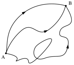
Three possible paths that the polymer can form starting from point A and ending at point B (unlike the diagram, the model described assumes constant contour length for all possible paths)

Under the same assumption of a smooth contour, the distribution function can be expressed using a path integral:

${\displaystyle \Phi ({\vec {R}},N)=\int _{0,0}^{{\vec {R}},N}\exp \left\{-\int _{0}^{N}L_{0}d\nu \right\}{\mathcal {D}}{\vec {R}}(\nu )}$

Where we defined ${\displaystyle \textstyle L_{0}={\frac {3}{2l^{2}}}\left({\frac {d{\vec {R}}}{d\nu }}\right)^{2}.}$

Here ${\displaystyle \nu }$ acts as a parametrization variable for the polymer, describing in effect its spatial configuration, or contour.

The exponent is a measure for the number density of polymer configurations in which the shape of the polymer is close to a continuous and differentiable curve. ^[3]

Spatial obstructions

Thus far, the path integral approach didn't avail us of any novel results. For that, one must venture further than the ideal model. As a first departure from this limited model, we now consider the constraint of spatial obstructions. The ideal model assumed no constraints on the spatial configuration of each additional monomer, including forces between monomers which obviously exist, since two monomers cannot occupy the same space. Here, we'll take the concept of obstruction to encompass not only monomer-monomer interactions, but also constraints that arise from the presence of dust and boundary conditions such as walls or other physical obstructions. ^[3]

Dust

Consider a space filled with small impenetrable particles, or "dust". Denote the fraction of space excluding a monomer end point by ${\displaystyle f({\vec {R}})}$ so its values range: ${\displaystyle 0\leq f({\vec {R}})\leq 1}$.

Constructing a Taylor expansion for ${\displaystyle \Phi ({\vec {R}},N+\Delta N).}$, one can arrive at the new governing differential equation:

${\displaystyle {\frac {\partial \Phi }{\partial N}}={\frac {l^{2}}{6}}\nabla ^{2}-f\Phi }$

For which the corresponding path integral is:

${\displaystyle \Phi ({\vec {R}},N)=\int _{0,0}^{{\vec {R}},N}\exp \left\{-\int _{0}^{N}[L_{0}+f({\vec {R}})]d\nu \right\}{\mathcal {D}}{\vec {R}}(\nu )}$

Walls

Diagram of a cell membrane. A common form of "wall" a polymer might encounter.

To model a perfect rigid wall, simply set ${\displaystyle \textstyle {\frac {f({\vec {R}})}{l^{2}}}\rightarrow +\infty }$ for all regions in space out of reach of the polymer due to the wall contour.

The walls a polymer usually interacts with are complex structures. Not only can the contour be full of bumps and twists, but their interaction with the polymer is far from the rigid mechanical idealization depicted above. In practice, a polymer will often be "absorbed" or condense on the wall due to attractive intermolecular forces. Due to heat, this process is counteracted by an entropy driven process, favoring polymer configurations that correspond to large volumes in phase space. A thermodynamic adsorption-desorption process arises. One common example for this are polymers confined within a cell membrane.

To account for the attraction forces, define a potential per monomer denoted as: ${\displaystyle \textstyle V({\vec {R}})}$. The potential will be incorporated through a Boltzmann factor. Taken for the entire polymer this takes the form:

${\displaystyle \exp \left\{-\beta \sum _{j=0}^{N}V({\vec {R}}_{j})\right\}\cong \exp \left\{-\beta \int _{0}^{N}V({\vec {R}}(\nu ))\right\}}$

Where we used ${\displaystyle \beta =(k_{b}T)^{-}1}$ with ${\displaystyle T}$ as Temperature and ${\displaystyle k_{b}}$ the Boltzmann constant. In the right hand side, our usual limits ${\displaystyle N\rightarrow \infty \quad \&\quad L\rightarrow 0}$ were taken.

The number of polymer configurations with fixed endpoints can now be determined by the path integral:

${\displaystyle Q_{V}({\vec {R}}_{N},N|{\vec {R}}_{0},0)=\int _{{\vec {R}}_{0},0}^{{\vec {R}}_{N},N}\exp \left\{-\int _{0}^{N}[L_{0}]d\nu \right\}{\mathcal {D}}{\vec {R}}(\nu )}$

Similarly to the ideal polymer case, this integral can be interpreted as a propagator for the differential equation:

${\displaystyle {\frac {\partial f}{\partial N}}={\frac {l^{2}}{6}}\nabla ^{2}f-\beta V({\vec {R}})f}$

This leads to a bi-linear expansion for ${\displaystyle Q_{V}({\vec {R}}_{N},N|{\vec {R}}_{0},0)=\sum _{n}f_{n}({\vec {R}}_{N})f_{n}^{*}({\vec {R}}_{0})\exp(-E_{N}N)}$ in terms of orthonormal eigenfunctions and eigenvalues:

${\displaystyle \left[{\frac {l^{2}}{6}}\nabla ^{2}f-\beta V({\vec {R}})\right]f_{n}({\vec {R}}_{n})=E+nf_{n}({\vec {R}}_{n})}$

and so our absorption problem is reduced to an eigenfunction problem.

For a typical well like (attractive) potential this leads to two regimes for the absorption phenomenon, with the critical temperature ${\displaystyle T_{c}}$ determined by the specific problem parameters ${\displaystyle l,V({\vec {R}})}$ :

In high temperatures ${\displaystyle T>T_{c}}$, the potential well has no bound states, meaning all eigenvalues are positive and the corresponding eigenfunction takes the asymptotic form ${\displaystyle <(x\rightarrow \infty )}$:

${\displaystyle f_{n}\cong A_{n}\sin({\sqrt {6\lambda _{n}/L^{2}}}x)+B_{m}\cos({\sqrt {6\lambda _{m}/L^{2}}}x)}$ with ${\displaystyle \lambda _{n}}$ denoting the calculated eigenvalues.

The result is shown for the x coordinate after a separation of variables and assuming a surface at ${\displaystyle x=0}$. This expression represents a very open configuration for the polymer, away from the surface, meaning the polymer is desorbed.

For low enough temperatures ${\displaystyle T<T_{c}}$, there exist at least one bounded state with a negative eigenvalue. In our "large polymer" limit, this means that the bi-linear expansion will be dominated by the ground state, which asymptotically ${\displaystyle (x\rightarrow \infty )}$ takes the form:

${\displaystyle f(x_{0})\cong A_{0}\exp(-{\sqrt {6|\lambda _{0}|/l^{2}}}x)}$

This time the configurations of the polymer are localized in a narrow layer near the surface with an effective thickness ${\displaystyle \textstyle {\frac {l}{\sqrt {6|\lambda _{0}|}}}}$

A wide variety of adsorption problems boasting a host of "wall" geometries and interaction potentials can be solved using this method. To obtain a quantitatively well defined result one has to use the recovered eigenfunctions and construct the corresponding configuration sum.

For a complete and rigorous solution see. ^[11]

Excluded volume

Another obvious obstruction, thus far blatantly disregarded, is the interactions between monomers within the same polymer. An exact solution for the number of configurations under this very realistic constraint has not yet been found for any dimension larger than one. ^[3] This problem has historically came to be known as the excluded volume problem. To better understand the problem, one can imagine a random walk chain, as previously presented, with a small hard sphere (not unlike the "specks of dust" mentioned above) at the endpoint of each monomer. The radius of these spheres necessarily obeys ${\displaystyle r<l/2}$, otherwise successive spheres would overlap.

A path integral approach affords a relatively simple method to derive an approximated solution: ^[12] The results presented are for three dimensional space, but can be easily generalized to any dimensionality. The calculation is based on two reasonable assumptions:

1. Statistical characteristics for the volume excluded case resemble that of a polymer without excluded volume but with a fraction ${\displaystyle f({\vec {R}})}$ occupied by small spheres of an identical volume to the hypothesized monomer sphere.
2. These aforementioned characteristics can be approximated by a calculation of the most probable chain configuration.

In accordance with the path integral expression for ${\displaystyle \textstyle Q_{V}({\vec {R}}_{N},N|{\vec {R}}_{0}.0)}$ previously presented, the most probable configuration will be the curve ${\displaystyle {\vec {R}}^{*}(\nu )}$ that minimizes the exponent of the original path integral:

${\displaystyle S[{\vec {R}}(\nu )]\equiv \int _{0}^{N}\left\{{\frac {3}{2l^{2}}}\left({\frac {d{\vec {R}}}{d\nu }}\right)^{2}+f({\vec {R}})\right\}d\nu }$

To minimize the expression, employ calculus of variations and obtain the Euler–Lagrange equation:

${\displaystyle {\frac {3}{l^{2}}}{\frac {d^{2}{\vec {R}}^{*}}{d\nu ^{2}}}=\nabla f({\vec {R}}^{*})}$

We set ${\displaystyle R\equiv R^{*}}$.

To determine the appropriate function ${\displaystyle f({\vec {R}})}$, consider a sphere of radius ${\displaystyle R}$, thickness ${\displaystyle dR}$ and profile ${\displaystyle 4\pi R^{2}}$ centered around the origin of the polymer. The average number of monomers in this shell should equal ${\displaystyle \textstyle {\frac {4\pi R^{2}}{(4/3)\pi r^{3}}}f(R)dR}$.

On the other hand, the same average should also equal ${\displaystyle \textstyle d\nu =\left({\frac {dR}{d\nu }}\right)^{-1}}$ (Remember that ${\displaystyle \nu }$ was defined as a parametrization factor with values ${\displaystyle 0\leq \nu \leq N}$). This equality results in:

${\displaystyle f({\vec {R}})={\frac {(4/3)\pi r^{3}}{4\pi }}R^{2}\left({\frac {dR}{d\nu }}\right)^{-1}}$

We find ${\displaystyle S[{\vec {R}}(\nu )]}$ can now be written as:

${\displaystyle S[{\vec {R}}(\nu )]=\int _{0}^{N}\left\{{\frac {3}{2l^{2}}}\left({\frac {dR}{d\nu }}\right)^{2}+{\frac {(4/3)\pi r^{3}}{4\pi }}R^{2}\left({\frac {dR}{d\nu }}\right)^{-1}\right\}d\nu }$

We again use variation calculus to arrive at:

${\displaystyle \left\{{\frac {3}{l^{2}}}+{\frac {2(4/3)\pi r^{3}}{4\pi }}R^{2}\left({\frac {dR}{d\nu }}\right)^{-3}\right\}{\frac {d^{2}R}{d\nu ^{2}}}+4{\frac {(4/3)\pi r^{3}}{4\pi }}R^{2}\left({\frac {dR}{d\nu }}\right)^{-1}=0}$

Note that we now have an ODE for ${\displaystyle R(\nu )}$ without any ${\displaystyle f({\vec {R}}^{*})}$ dependence. Although quite horrendous to look at, this equation has a fairly simple solution:

${\displaystyle R(\nu )=\left({\frac {3\pi }{(4/3)\pi r^{3}L^{2}}}\right)^{-1/5}\left({\frac {3}{5}}\right)^{-3/5}\nu ^{3/5}}$

We arrived at the important conclusion that for a polymer with excluded volume the end to end distance grows with N like:

${\displaystyle R\cong \left({\frac {3\pi }{(4/3)\pi r^{3}L^{2}}}\right)^{-1/5}N^{3/5}}$, a first departure from the ideal model result: ${\displaystyle R\sim {\sqrt {N}}}$.

Gaussian chain

Conformational distribution

So far, the only polymer parameters incorporated into the calculation were the number of monomers ${\displaystyle N}$ which was taken to infinity, and the constant bond length ${\displaystyle l}$. This is usually sufficient, as that is the only way the local structure of the polymer affects the problem. To try and do a bit better than the "constant bond distance" approximation, let us examine the next most rudimentary approach; A more realistic description of the single bond length will be a Gaussian distribution: ^[13]

${\displaystyle \psi ({\vec {r}})=\left({\frac {3}{2\pi l^{2}}}\right)^{3/2}\exp \left(-{\frac {3{\vec {r}}^{2}}{2l^{2}}}\right)}$

So like before, we maintain the result: ${\displaystyle \langle {\vec {r}}^{2}\rangle =l^{2}}$. Note that although a bit more complex than before, ${\displaystyle \psi ({\vec {r}})}$ still has a single parameter - ${\displaystyle l}$.

The conformational distribution function for our new bond vector distribution is:

${\displaystyle {\begin{aligned}\Psi (\left\{{\vec {r}}_{n}\right\})&=\prod _{n=1}^{N}\psi ({\vec {r}}_{n})\\&=\prod _{n=1}^{N}\left({\frac {3}{2\pi l^{2}}}\right)^{3/2}\exp \left[-{\frac {3{\vec {r}}_{n}^{2}}{2l^{2}}}\right]\\&=\left({\frac {3}{2\pi l^{2}}}\right)^{3N/2}\exp \left[-\sum _{n=1}^{N}{\frac {3({\vec {R}}_{n}-{\vec {R}}_{n-1})^{2}}{2l^{2}}}\right].\end{aligned}}}$

Where we switched from the relative bond vector ${\displaystyle {\vec {r}}_{n}}$ to the absolute position vector difference: ${\displaystyle ({\vec {R}}_{n}-{\vec {R}}_{n-1})}$.

This conformation is known as the Gaussian chain. The Gaussian approximation for ${\displaystyle \psi ({\vec {r}})}$ does not hold for a microscopic analysis of the polymer structure but will yield accurate results for large-scale properties.

An intuitive way to construe this model is as a mechanical model of beads successively connected by a harmonic spring. The potential energy for such a model is given by:

${\displaystyle U_{0}(\{{\vec {R}}_{n}\})={\frac {3}{2l^{2}}}k_{b}T\sum _{n=1}^{N}({\vec {R}}_{n}-{\vec {R}}_{n-1})}$

At thermal equilibrium one can expect the Boltzmann distribution, which indeed recovers the result above for ${\displaystyle \Psi (\left\{{\vec {r}}_{n}\right\})}$.

An important property of the Gaussian chain is self-similarity. Meaning the distribution for ${\displaystyle {\vec {R}}_{n}-{\vec {R}}_{m}}$ between any two units is again Gaussian, depending only on ${\displaystyle l}$ and the unit to unit distance ${\displaystyle (n-m)}$:

${\displaystyle \phi ({\vec {R}}_{n}-{\vec {R}}_{m}|n-m)=\left({\frac {3}{2\pi l^{2}|n-m|}}\right)^{3/2}\exp \left[-{\frac {3({\vec {R}}_{n}-{\vec {R}}_{m})^{2}}{2|n-m|l^{2}}}\right]}$

This immediately leads to ${\displaystyle <({\vec {R}}_{n}-{\vec {R}}_{m})^{2}>=|n-m|l^{2}}$.

As was implicitly done in the section for spatial obstructions, we take the suffix ${\displaystyle n}$ to a continuous limit and replace ${\displaystyle {\vec {R}}_{n}-{\vec {R}}_{m}}$ by ${\displaystyle \partial {\vec {R}}_{n}/\partial n}$. So now, our conformational distribution is expressed by:

${\displaystyle \Psi (\left\{{\vec {r}}_{n}\right\})=\left({\frac {3}{2\pi l^{2}}}\right)^{3N/2}\exp \left[-{\frac {3}{2l^{2}}}\int _{0}^{N}dn\left({\frac {\partial {\vec {R}}_{n}}{\partial n}}\right)^{2}\right].}$

The independent variable transformed from a vector into a function, meaning ${\displaystyle \Psi [{\vec {R}}(n)]}$ is now a functional. This formula is known as the Wiener distribution.

Chain conformation under an external field

Assuming an external potential field ${\displaystyle U_{e}({\vec {R}})}$, the equilibrium conformational distribution described above will be modified by a Boltzmann factor:

${\displaystyle \Psi (\left\{{\vec {r}}_{n}\right\})=\left({\frac {3}{2\pi l^{2}}}\right)^{3N/2}\exp \left[-{\frac {3}{2l^{2}}}\int _{0}^{N}dn\left({\frac {\partial {\vec {R}}_{n}}{\partial n}}\right)^{2}-\beta \int _{0}^{N}dnU_{e}[{\vec {R}}(n)]\right].}$

An important tool in the study of a Gaussian chain conformational distribution is the Green function, defined by the path integral quotient:

${\displaystyle G({\vec {R}},{\vec {R}}';N)\equiv {\frac {\displaystyle \int _{{\vec {R}}_{0}={\vec {R}}'}^{{\vec {R}}_{N}={\vec {R}}}{\mathcal {D}}{\vec {R}}(n)\exp \left[-{\frac {3}{2l^{2}}}\displaystyle \int _{0}^{N}dn\left({\frac {\partial {\vec {R}}_{n}}{\partial n}}\right)^{2}-\beta \displaystyle \int _{0}^{N}duU_{e}[{\vec {R}}(n)]\right]}{\displaystyle \int d{\vec {R}}'\displaystyle \int d{\vec {R}}\displaystyle \int _{{\vec {R}}_{0}={\vec {R}}'}^{{\vec {R}}_{N}={\vec {R}}}{\mathcal {D}}{\vec {R}}_{n}\exp \left[-{\frac {3}{2l^{2}}}\displaystyle \int _{0}^{N}dn\left({\frac {\partial {\vec {R}}_{n}}{\partial n}}\right)^{2}\right]}}}$

The path integration is interpreted as a summation over all polymer curves ${\displaystyle {\vec {R}}(n)}$ that start from ${\displaystyle {\vec {R}}_{0}={\vec {R}}'}$ and terminate at ${\displaystyle {\vec {R}}_{N}={\vec {R}}}$.

For the simple zero field case ${\displaystyle U_{e}=0}$ The Green function reduces back to:

${\displaystyle G({\vec {R}}-{\vec {R}}';N)=\left({\frac {3}{2\pi l^{2}N}}\right)^{3/2}\exp \left[-{\frac {3({\vec {R}}-{\vec {R}}')^{2}}{2Nl^{2}}}\right]}$

In the more general case, ${\displaystyle G({\vec {R}}-{\vec {R}}';N)}$ plays the role of a weight factor in the complete partition function for all possible polymer conformations:

${\displaystyle Z=\int d{\vec {R}}~d{\vec {R}}'~G({\vec {R}}-{\vec {R}}';N).}$

There exists an important identity for the Green function that stems directly from its definition:

${\displaystyle G({\vec {R}},{\vec {R}}';N)=\int d{\vec {R}}''G({\vec {R}},{\vec {R}}'';N-n)G({\vec {R}}'',{\vec {R}}';N),\quad (0<n<N).}$

This equation has a clear physical significance, which might also serve to elucidate the concept of the path integral:

The product ${\displaystyle \textstyle G({\vec {R}},{\vec {R}}'';N-n)G({\vec {R}}'',{\vec {R}}';N))}$ expresses the weight factor for a chain which starts at ${\displaystyle R'}$, passes through ${\displaystyle R''}$ in ${\displaystyle n}$ steps, and ends at ${\displaystyle R}$ after ${\displaystyle N}$ steps. The integration over all possible midpoints ${\displaystyle R''}$ gives back the statistical weight for a chain starting at ${\displaystyle R'}$, and terminating at ${\displaystyle R}$. It should now be clear that the path integral is simply a sum over all possible literal paths the polymer can form between two fixed endpoints.

With the help of ${\displaystyle G({\vec {R}},{\vec {R}}';N)}$ the average of any physical quantity ${\displaystyle A}$ can be calculated. Assuming ${\displaystyle \textstyle A}$ depends only on the position of the ${\displaystyle n}$-th segment, then:

${\displaystyle \left\langle A({\vec {R}}_{n})\right\rangle ={\frac {\displaystyle \int d{\vec {R}}_{N}~d{\vec {R}}_{n}~d{\vec {R}}_{0}~G({\vec {R}}_{N},{\vec {R}}_{n};N-n)G({\vec {R}}_{n},{\vec {R}}_{0};n)A({\vec {R}}_{n})}{\displaystyle \int d{\vec {R}}_{N}~{\vec {d}}R_{0}~G({\vec {R}}_{N},{\vec {R}}_{0};N)}}}$

It stands to reason that A should depend on more than one monomer. assuming now it depends on ${\displaystyle {\vec {R}}_{m}}$ as well as ${\displaystyle {\vec {R}}_{n}}$ the average takes the form:

${\displaystyle \left\langle A({\vec {R}}_{n},{\vec {R}}_{m})\right\rangle ={\frac {\displaystyle \int d{\vec {R}}_{N}~d{\vec {R}}_{n}~d{\vec {R}}_{m}~d{\vec {R}}_{0}~G({\vec {R}}_{N},{\vec {R}}_{n};N-n)G({\vec {R}}_{n},{\vec {R}}_{m};n-m)A({\vec {R}}_{n},{\vec {R}}_{m})}{\displaystyle \int d{\vec {R}}_{N}~{\vec {d}}R_{0}~G({\vec {R}}_{N},{\vec {R}}_{0};N)}}}$

With an obvious generalization for more monomers dependence.

If one imposes the reasonable boundary conditions:

${\displaystyle {\begin{aligned}&G({\vec {R}},{\vec {R}}';N<0)=0\\&G({\vec {R}},{\vec {R}}';0)=\delta ({\vec {R}}-{\vec {R}}')\\\end{aligned}}}$

then with the help of a Taylor expansion for ${\displaystyle G({\vec {R}},{\vec {R}}';N+\Delta N)}$, a differential equation for ${\displaystyle G}$ can be derived:

${\displaystyle \left({\frac {\partial }{\partial N}}-{\frac {l^{2}}{6}}{\frac {\partial ^{2}}{\partial {\vec {R}}^{2}}}+\beta U_{e}({\vec {R}}))\right)G({\vec {R}},{\vec {R}}';N)=\delta ^{3}({\vec {R}}-{\vec {R}}')\delta (N).}$

With the help of this equation the explicit form of ${\displaystyle G({\vec {R}},{\vec {R}}';N)}$ is found for a variety of problems. Then, with a calculation of the partition function a host of statistical quantities can be extracted.

Polymer field theory

Main article: Polymer field theory

A different new approach for finding the power dependence ${\displaystyle \left\langle {\vec {R}}^{2}\right\rangle \propto N^{\alpha }}$ caused by excluded volume effects, is considered superior to the one previously presented. ^[6]

The field theory approach in polymer physics is based on an intimate relationship of polymer fluctuations and field fluctuations. The statistical mechanics of a many particle system can be described by a single fluctuating field. A particle in such an ensemble moves through space along a fluctuating orbit in a fashion that resembles a random polymer chain. The immediate conclusion to be drawn is that large groups of polymers may also be described by a single fluctuating field. As it turns out, the same can be said of a single polymer as well.

In analogy to the original path integral expression presented, the end to end distribution of the polymer now takes the form:

${\displaystyle \Phi ({\vec {R}},N)=\int _{0,0}^{{\vec {R}},N}e^{-{\mathcal {A}}[\eta ]}P^{\eta }(N,l){\mathcal {D}}\eta }$

Our new path integrand consists of:

• The fluctuating field ${\displaystyle \eta ({\vec {R}})}$
• The action  :${\displaystyle {\mathcal {A}}[\eta ]=-{\frac {1}{2}}\int d{\vec {R}}~d{\vec {R}}'~\eta ({\vec {R}})V^{-1}({\vec {R}},{\vec {R}}')\eta ({\vec {R}}')}$ with ${\displaystyle V({\vec {R}},{\vec {R}}')}$ denoting the monomer-monomer repulsive potential.
• ${\displaystyle P^{\eta }(N,L)=\int \exp \left\{-\int _{0}^{N}d\nu \left[{\frac {M}{2}}{\dot {\vec {R}}}+\eta ({\vec {R}}(\nu ))\right]\right\}{\mathcal {D}}{\vec {R}}}$ which satisfies the Schrödinger equation:

${\displaystyle \left[{\frac {\partial }{\partial N}}-{\frac {1}{2M}}\nabla ^{2}+\eta ({\vec {R}})\right]P^{\eta }(N,L)=\delta ^{(3)}({\vec {R}}-{\vec {R}}')\delta (N)}$ with ${\displaystyle M}$ acting as an effective mass determined by the dimensionality and bond length.

Note that the inner integral is now also a path integral, so two spaces of function are integrated over - the polymer conformations - ${\displaystyle {\vec {R}}(\nu )}$ and the scalar fields ${\displaystyle \eta ({\vec {R}})}$.

These path integrals have a physical interpretation. The action ${\displaystyle {\mathcal {A}}}$ describes the orbit of a particle in a space dependent random potential ${\displaystyle \eta ({\vec {R}})}$. The path integral over ${\displaystyle {\vec {R}}(\nu )}$ yields the end to end distribution of the fluctuating polymer in this potential. The second path integral over ${\displaystyle \eta ({\vec {R}})}$ with the weight ${\displaystyle e^{-{\mathcal {A}}[\eta ]}}$ accounts for the repulsive cloud of other chain elements. To avoid divergence, the ${\displaystyle \eta ({\vec {R}})}$ integration has to run along the imaginary field axis.

Such a field description for a fluctuating polymer has the important advantage that it establishes a connection with the theory of critical phenomena in field theory.

To find a solution for ${\displaystyle \Phi ({\vec {R}},N)}$, one usually employs a Laplace transform and considers a correlation function similar to the statistic average ${\displaystyle \left\langle A({\vec {R}}_{n},{\vec {R}}_{m})\right\rangle }$ formerly described, with the green function substituted by a fluctuating complex field. In the common limit of large polymers (N>>1), the solutions for the end to end vector distribution correspond to the well developed regime studied in the quantum field theoretic approach to critical phenomena in many body systems. ^{[14] [15]}

Many-polymer systems

Another simplifying assumption was taken for granted in the treatment presented thus far; All models described a single polymer. Obviously a more physically realistic description will have to account for the possibility of interactions between polymers. In essence, this is an extension of the excluded volume problem.

To see this from a pictorial point, one can imagine a snap shot of a concentrated polymer solution. Excluded volume correlations are now not only taking place within one single chain, but an increasing number of contact points from other chains at increasing polymer concentration yields additional excluded volume. These additional contacts can have substantial effects on the statistical behavior of the individual polymer.

A distinction must be made between two different length scales. ^[16] One regime will be given by small end to end vector scales ${\displaystyle R_{0}<\xi }$. At these scales the chain piece experiences only correlations from itself, i.e., the classical self-avoiding behavior. For larger scales ${\displaystyle R_{0}>\xi }$ self-avoiding correlations do not play a significant role and the chain statistics resemble a Gaussian chain. The critical value ${\displaystyle \xi }$ must be a function of the concentration. Intuitively, one significant concentration can already be found. This concentration characterizes the overlap between the chains. If the polymers just marginally overlap, one chain is occupied in its own volume. This gives:

${\displaystyle C^{*}=N/R_{0}^{3}\sim N/N^{3\sigma }=N^{1-3\sigma }}$ Where we used ${\displaystyle R_{0}\sim N^{\sigma }}$

This is an important result and one immediately sees that for large chain lengths N, the overlap concentration is very small. The self-avoiding walk previously described is changed and therefore the partition function is no longer ruled by the single polymer volume excluded paths, but by the remaining density fluctuations which are determined by the overall concentration of the polymer solution. In the limit of very large concentrations, imagined by an almost completely filled lattice, the density fluctuations become less and less important.

To begin with, let us generalize the path integral formulation to many chains. The generalization for the partition function calculation is very simple and all that has to be done is to take into account the interaction between all the chain segments:

${\displaystyle Z=\int \prod _{\alpha =1}^{n_{p}}{\mathcal {D}}{\vec {R}}_{\alpha }(\nu )\exp\{-\beta {\mathcal {H}}([{\vec {R}}_{\alpha }(\nu )])\}}$

Where the weighed energy states are defined as:

${\displaystyle \displaystyle \beta {\mathcal {H}}([{\vec {R}}_{\alpha }(\nu )])={\frac {3}{2l^{2}}}\sum _{\alpha =1}^{n_{p}}\int _{0}^{N_{\alpha }}\left({\frac {\partial {\vec {R}}_{\alpha }}{\partial \nu }}\right)^{2}d\nu +{\frac {1}{2}}\sigma \sum _{\alpha ,\beta =1}^{n_{p}}\int _{0}^{N_{\alpha }}d\nu \int _{0}^{N_{\beta }}d\nu '\delta ({\vec {R}}_{\alpha }(\nu )-{\vec {R}}_{\beta }(\nu '))}$

With ${\displaystyle n_{p}}$ denoting the number of polymers.

This is generally not simple and the partition function cannot be computed exactly. One simplification is to assume monodispersity which means that all chains have the same length. or, mathematically: ${\displaystyle N_{\alpha }=N_{\beta }\quad \forall \ \alpha ,\beta }$.

Another problem is that the partition function contains too many degrees of freedom. The number of chains ${\displaystyle n_{p}}$ involved can be very large and every chain has internal degrees of freedom, since they are assumed to be totally flexible. For this reason, it is convenient to introduce collective variables, which in this case is the polymer segment density:

${\displaystyle \rho ({\vec {x}})={\frac {1}{V}}\sum _{\alpha =1}^{n_{p}}\int _{0}^{N}d\nu \delta ({\vec {x}}-{\vec {R}}_{\alpha }(\nu )).}$ with ${\displaystyle V}$ the total solution volume.

${\displaystyle \rho ({\vec {x}})}$ can be viewed as a microscopic density operator whose value defines the density at an arbitrary point ${\displaystyle {\vec {x}}}$.

The transformation ${\displaystyle {\mathcal {H}}([{\vec {R}}_{\alpha }(\nu )])\rightarrow {\mathcal {H}}([\rho ({\vec {x}})])}$ is less trivial than one might imagine and cannot be carried out exactly. The final result corresponds to the so-called random phase approximation (RPA) which has been frequently used in solid-state physics. To explicitly calculate the partition function using the segment density one has to switch to reciprocal space, change variables and only then execute the integration. For a detailed derivation see. ^{[13] [17]} With the partition function obtained, a variety of physical quantities can be extracted as previously described.

See also

• File dynamics
• Kuhn length
• Important publications in polymer physics
• Persistence length
• Polymer characterization
• Random coil
• Worm-like chain

References

1. H.R Allcock; F.W. Lampe; J.E Mark, Contemporary Polymer Chemistry (3 ed.). (Pearson Education 2003). p. 21. ISBN   0-13-065056-0.
2. P. Flory, Principles of Polymer Chemistry, Cornell University Press, 1953. ISBN   0-8014-0134-8.
3. F.W. Wiegel, Introduction to Path-Integral Methods in Physics and Polymer science (World Scientific, Philadelphia, 1986).
4. Doi, Masao; Edwards, S. F. (1978). "Dynamics of concentrated polymer systems. Part 1—3". J. Chem. Soc., Faraday Trans. 2. Royal Society of Chemistry (RSC). 74: 1789–1832. doi:10.1039/f29787401789. ISSN   0300-9238.
5. Doi, Masao; Edwards, S. F. (1979). "Dynamics of concentrated polymer systems. Part 4.—Rheological properties". J. Chem. Soc., Faraday Trans. 2. Royal Society of Chemistry (RSC). 75: 38–54. doi:10.1039/f29797500038. ISSN   0300-9238.
6. H. Kleinert, PATH INTEGRALS in Quantum mechanics, Statistics, Polymer Physics, and Financial Markets (World Scientific, 2009).
7. Daniell, P. J. (1918). "A General Form of Integral". The Annals of Mathematics. JSTOR. 19 (4): 279–294. doi: 10.2307/1967495 . ISSN   0003-486X. JSTOR   1967495.
8. Wiener, N. (1 August 1921). "The Average of an Analytic Functional". Proceedings of the National Academy of Sciences. 7 (9): 253–260. Bibcode:1921PNAS....7..253W. doi: 10.1073/pnas.7.9.253 . ISSN   0027-8424. PMC   1084890 . PMID   16576602.
9. R.P. Feynman, "The Principle of Least Action in quantum Mechanics," Pd.d Thesis, Princeton University (1942), unpublished.
10. R.P. Feynman and A.R. Hibbs, Quantum Mechanics and Path Integrals (McGraw-Hill, New York, 1965).
11. Rubin, Robert J. (15 November 1969). "Comment on "Conformation of Adsorbed Polymeric Chain. II"". The Journal of Chemical Physics. AIP Publishing. 51 (10): 4681. Bibcode:1969JChPh..51.4681R. doi: 10.1063/1.1671849 . ISSN   0021-9606.
12. Gennes, P -G de (1 December 1968). "Some conformation problems for long macromolecules". Reports on Progress in Physics. IOP Publishing. 32 (1): 187–205. doi:10.1088/0034-4885/32/1/304. ISSN   0034-4885. S2CID   250861107.
13. M. Doi and S.F. Edwards, The Theory of Polymer Dynamics, (Clarendon press,Oxford, 1986).
14. D.J. Amit, Renormalization Group and Critical Phenomena, (World Scientific Singapore, 1984.)
15. G. Parisi, Statistical Field Theory, (Addison-Wesley, Reading Mass. 1988).
16. Vilgis, T.A. (2000). "Polymer Theory: Path Integrals and Scaling". Physics Reports. 336 (3): 167–254. Bibcode:2000PhR...336..167V. doi:10.1016/S0370-1573(99)00122-2.
17. Edwards, S F; Anderson, P W (1975). "Theory of spin glasses". Journal of Physics F: Metal Physics. IOP Publishing. 5 (5): 965–974. Bibcode:1975JPhF....5..965E. doi:10.1088/0305-4608/5/5/017. ISSN   0305-4608.