Fractal tree index

Last updated
Fractal tree index
Type tree
Invented2007
Invented by Michael A. Bender, Martin Farach-Colton, Bradley C. Kuszmaul
Time complexity in big O notation
AlgorithmAverageWorst case
SpaceO(N/B)O(N/B)
SearchO(logBN)O(logBN)
InsertO(logBN/Bε)O(logBN/Bε)
DeleteO(logBN/Bε)O(logBN/Bε)

In computer science, a fractal tree index is a tree data structure that keeps data sorted and allows searches and sequential access in the same time as a B-tree but with insertions and deletions that are asymptotically faster than a B-tree. Like a B-tree, a fractal tree index is a generalization of a binary search tree in that a node can have more than two children. Furthermore, unlike a B-tree, a fractal tree index has buffers at each node, which allow insertions, deletions and other changes to be stored in intermediate locations. The goal of the buffers is to schedule disk writes so that each write performs a large amount of useful work, thereby avoiding the worst-case performance of B-trees, in which each disk write may change a small amount of data on disk. Like a B-tree, fractal tree indexes are optimized for systems that read and write large blocks of data. The fractal tree index has been commercialized in databases by Tokutek. Originally, it was implemented as a cache-oblivious lookahead array, [1] but the current implementation is an extension of the Bε tree. [2] The Bε is related to the Buffered Repository Tree. [3] The Buffered Repository Tree has degree 2, whereas the Bε tree has degree Bε. The fractal tree index has also been used in a prototype filesystem. [4] [5] An open source implementation of the fractal tree index is available, [6] which demonstrates the implementation details outlined below.

Contents

Overview

In fractal tree indexes, internal (non-leaf) nodes can have a variable number of child nodes within some pre-defined range. When data is inserted or removed from a node, its number of child nodes changes. In order to maintain the pre-defined range, internal nodes may be joined or split. Each internal node of a B-tree will contain a number of keys that is one less than its branching factor. The keys act as separation values which divide its subtrees. Keys in subtrees are stored in search tree order, that is, all keys in a subtree are between the two bracketing values. In this regard, they are just like B-trees.

Fractal tree indexes and B-trees both exploit the fact that when a node is fetched from storage, a block of memory, whose size is denoted by , is fetched. Thus, nodes are tuned to be of size approximately . Since access to storage can dominate the running time of a data structure, the time-complexity of external memory algorithms is dominated by the number of read/writes a data structure induces. (See, e.g., [7] for the following analyses.)

In a B-tree, this means that the number of keys in a node is targeted to be enough to fill the node, with some variability for node splits and merges. For the purposes of theoretical analysis, if keys fit in a node, then the tree has depth , and this is the I/O complexity of both searches and insertions.

Fractal trees nodes use a smaller branching factor, say, of . The depth of the tree is then , thereby matching the B-tree asymptotically. The remaining space in each node is used to buffer insertions, deletion and updates, which we refer to in aggregate as messages. When a buffer is full, it is flushed to the children in bulk. There are several choices for how the buffers are flushed, all leading to similar I/O complexity. Each message in a node buffer will be flushed to a particular child, as determined by its key. Suppose, for concreteness, that messages are flushed that are heading to the same child, and that among the children, we pick the one with the most messages. Then there are at least messages that can be flushed to the child. Each flush requires flushes, and therefore the per-message cost of a flush is .

Consider the cost of an insertion. Each message gets flushed times, and the cost of a flush is . Therefore, the cost of an insertion is . Finally, note that the branching factor can vary, but for any branching factor , the cost of a flush is , thereby providing a smooth tradeoff between search cost, which depends on the depth of the search tree, and therefore the branching factor, versus the insertion time, which depends on the depth of the tree but more sensitively on the size of the buffer flushes.

Comparisons with other external-memory indexes

This section compares fractal tree indexes with other external memory indexing data structures. The theoretical literature on this topic is very large, so this discussion is limited to a comparison with popular data structures that are in use in databases and file systems.

B-trees

The search time of a B-tree is asymptotically the same as that of a fractal tree index. However, a fractal tree index has deeper trees than a B-tree, and if each node were to require an I/O, say if the cache is cold, then a fractal tree index would induce more IO. However, for many workloads most or all internal nodes of both B-trees and fractal tree indexes are already cached in RAM. In this case, the cost of a search is dominated by the cost of fetching the leaf, which is the same in both cases. Thus, for many workloads, fractal tree indexes can match B-trees in terms of search time.

Where they differ is on insertions, deletions and updates. An insertion in a fractal tree index takes whereas B-trees require . Thus, fractal tree indexes are faster than B-trees by a factor of . Since can be quite large, this yields a potential two-order-of-magnitude improvement in worst-case insertion times, which is observed in practice. Both B-trees and fractal tree indexes can perform insertions faster in the best case. For example, if keys are inserted in sequential order, both data structures achieve a I/Os per insertion. Thus, because the best and worst cases of B-trees differ so widely, whereas fractal tree indexes are always near their best case, the actual speedup that fractal tree indexes achieve over B-trees depends on the details of the workload.

Log-structured merge-trees

Log-structured merge-trees (LSMs) refer to a class of data structures which consists of two or more index structures of exponentially growing capacities. When a tree at some level reaches its capacity, it is merged into the next bigger level. The IO-complexity of an LSM depends on parameters such as the growth factor between levels and the data structure chosen at each level, so in order to analyze the complexity of LSMs, we need to pick a specific version. For comparison purposes, we select the version of LSMs that match fractal tree indexes on insertion performance.

Suppose an LSM is implemented via B-trees, each of which has a capacity that is larger than its predecessor. The merge time depends on three facts: The sorted order of keys in an -item B-tree can be produced in IOs; Two sorted lists of and items can be merged into a sorted list in IOs; and a B-tree of a sorted list of items can be built in IOs. When a tree overflows, it is merged into a tree whose size is larger, therefore a level that holds items requires IOs to merge. An item may be merged once per level, giving a total time of , which matches the fractal tree index.

The query time is simply the B-tree query time at each level. The query time into the th level is , since the th level has capacity . The total time is therefore . This is larger than both the B-tree and fractal tree indexes by a logarithmic factor. In fact, although B-trees and fractal tree indexes are both on the optimal tradeoff curve between insertions and queries, LSMs are not. They are incomparable with B-trees and are dominated by fractal tree indexes.

A few notes about LSMs: there are ways to make the queries faster. For example, if only membership queries are required and no successor/predecessor/range queries are, then Bloom filters can be used to speed up queries. Also, the growth factor between levels can be set to some other value, giving a range of insertion/query tradeoffs. However, for every choice of insertion rate, the corresponding fractal tree index has faster queries.

Bε trees

The fractal tree index is a refinement of the Bε tree. Like a Bε tree, it consists of nodes with keys and buffers and realizes the optimal insertion/query tradeoff. The fractal tree index differs in including performance optimization and in extending the functionality. Examples of improved functionality include ACID semantics. B-tree implementations of ACID semantics typically involve locking rows that are involved in an active transactions. Such a scheme works well in a B-tree because both insertions and queries involve fetching the same leaf into memory. Thus, locking an inserted row does not incur an IO penalty. However, in fractal tree indexes, insertions are messages, and a row may reside in more than one node at the same time. Fractal tree indexes therefore require a separate locking structure that is IO-efficient or resides in memory in order to implement the locking involved in implementing ACID semantics.

Fractal tree indexes also have several performance optimizations. First, buffers are themselves indexed in order to speed up searches. Second, leaves are much larger than in B-trees, which allows for greater compression. In fact, the leaves are chosen to be large enough that their access time is dominated by the bandwidth time, and therefore amortizes away the seek and rotational latency. Large leaves are an advantage with large range queries but slow down point queries, which require accessing a small portion of the leaf. The solution implemented in fractal tree indexes is to have large leaves that can be fetched as a whole for fast range queries but are broken into smaller pieces call basement nodes which can be fetched individually. Accessing a basement node is faster than accessing a leaf, because of the reduced bandwidth time. Thus the substructure of leaves in fractal tree indexes, as compared to Bε trees allows both range and point queries to be fast.

Messaging and fractal tree indexes

Insertions, deletions and updates are inserted as message into buffers that make their way towards the leaves. The messaging infrastructure can be exploited to implement a variety of other operations, some of which are discussed below.

Upserts

An upsert is a statement that inserts a row if it does not exist and updates it if it does. In a B-tree, an upsert is implemented by first searching for the row and then implementing an insertion or an update, depending on the result of the search. This requires fetching the row into memory if it is not already cached. A fractal tree index can implement an upsert by inserting a special upsert message. Such a message can, in theory, implement arbitrary pieces of code during the update. In practice, four update operations are supported:

  1. (a generalized increment)
  2. (a generalized decrement)
  3. (a decrement with a floor at 0)

These correspond to the update operations used in LinkBench, [8] a benchmark proposed by Facebook. By avoiding the initial search, upsert messages can improve the speed of upserts by orders of magnitude.

Schema changes

So far, all message types have modified single rows. However, broadcast messages, which are copied to all outgoing buffers, can modify all rows in a database. For example, broadcast messages can be used to change the format of all rows in a database. Although the total work required to change all rows is unchanged over the brute-force method of traversing the table, the latency is improved, since, once the message is injected into the root buffer, all subsequent queries will be able to apply the schema modification to any rows they encounter. The schema change is immediate and the work is deferred to such a time when buffers overflow and leaves would have gotten updated anyway.

Implementations

The fractal tree index has been implemented and commercialized by Tokutek. It is available as TokuDB as a storage engine for MySQL and MariaDB, and as TokuMX, a more complete integration with MongoDB. Fractal tree indexes have also been used in prototype filesystems, TokuFS [4] and BetrFS. [5]

Related Research Articles

<span class="mw-page-title-main">AVL tree</span> Self-balancing binary search tree

In computer science, an AVL tree is a self-balancing binary search tree. In an AVL tree, the heights of the two child subtrees of any node differ by at most one; if at any time they differ by more than one, rebalancing is done to restore this property. Lookup, insertion, and deletion all take O(log n) time in both the average and worst cases, where is the number of nodes in the tree prior to the operation. Insertions and deletions may require the tree to be rebalanced by one or more tree rotations.

<span class="mw-page-title-main">Binary search algorithm</span> Search algorithm finding the position of a target value within a sorted array

In computer science, binary search, also known as half-interval search, logarithmic search, or binary chop, is a search algorithm that finds the position of a target value within a sorted array. Binary search compares the target value to the middle element of the array. If they are not equal, the half in which the target cannot lie is eliminated and the search continues on the remaining half, again taking the middle element to compare to the target value, and repeating this until the target value is found. If the search ends with the remaining half being empty, the target is not in the array.

<span class="mw-page-title-main">Heap (data structure)</span> Computer science data structure

In computer science, a heap is a specialized tree-based data structure that satisfies the heap property: In a max heap, for any given node C, if P is a parent node of C, then the key of P is greater than or equal to the key of C. In a min heap, the key of P is less than or equal to the key of C. The node at the "top" of the heap is called the root node.

<span class="mw-page-title-main">Trie</span> K-ary search tree data structure

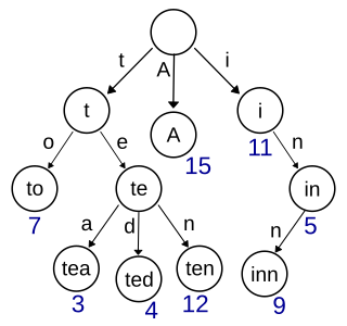
In computer science, a trie, also called digital tree or prefix tree, is a type of k-ary search tree, a tree data structure used for locating specific keys from within a set. These keys are most often strings, with links between nodes defined not by the entire key, but by individual characters. In order to access a key, the trie is traversed depth-first, following the links between nodes, which represent each character in the key.

<span class="mw-page-title-main">Binary heap</span> Variant of heap data structure

A binary heap is a heap data structure that takes the form of a binary tree. Binary heaps are a common way of implementing priority queues. The binary heap was introduced by J. W. J. Williams in 1964, as a data structure for heapsort.

<span class="mw-page-title-main">Treap</span>

In computer science, the treap and the randomized binary search tree are two closely related forms of binary search tree data structures that maintain a dynamic set of ordered keys and allow binary searches among the keys. After any sequence of insertions and deletions of keys, the shape of the tree is a random variable with the same probability distribution as a random binary tree; in particular, with high probability its height is proportional to the logarithm of the number of keys, so that each search, insertion, or deletion operation takes logarithmic time to perform.

In computer science, a skip list is a probabilistic data structure that allows average complexity for search as well as average complexity for insertion within an ordered sequence of elements. Thus it can get the best features of a sorted array while maintaining a linked list-like structure that allows insertion, which is not possible with a static array. Fast search is made possible by maintaining a linked hierarchy of subsequences, with each successive subsequence skipping over fewer elements than the previous one. Searching starts in the sparsest subsequence until two consecutive elements have been found, one smaller and one larger than or equal to the element searched for. Via the linked hierarchy, these two elements link to elements of the next sparsest subsequence, where searching is continued until finally searching in the full sequence. The elements that are skipped over may be chosen probabilistically or deterministically, with the former being more common.

In computing, a persistent data structure or not ephemeral data structure is a data structure that always preserves the previous version of itself when it is modified. Such data structures are effectively immutable, as their operations do not (visibly) update the structure in-place, but instead always yield a new updated structure. The term was introduced in Driscoll, Sarnak, Sleator, and Tarjans' 1986 article.

In computer science, a disjoint-set data structure, also called a union–find data structure or merge–find set, is a data structure that stores a collection of disjoint (non-overlapping) sets. Equivalently, it stores a partition of a set into disjoint subsets. It provides operations for adding new sets, merging sets, and finding a representative member of a set. The last operation makes it possible to find out efficiently if any two elements are in the same or different sets.

A B+ tree is an m-ary tree with a variable but often large number of children per node. A B+ tree consists of a root, internal nodes and leaves. The root may be either a leaf or a node with two or more children.

In data processing R*-trees are a variant of R-trees used for indexing spatial information. R*-trees have slightly higher construction cost than standard R-trees, as the data may need to be reinserted; but the resulting tree will usually have a better query performance. Like the standard R-tree, it can store both point and spatial data. It was proposed by Norbert Beckmann, Hans-Peter Kriegel, Ralf Schneider, and Bernhard Seeger in 1990.

In computer science, an interval tree is a tree data structure to hold intervals. Specifically, it allows one to efficiently find all intervals that overlap with any given interval or point. It is often used for windowing queries, for instance, to find all roads on a computerized map inside a rectangular viewport, or to find all visible elements inside a three-dimensional scene. A similar data structure is the segment tree.

In computer science, weight-balanced binary trees (WBTs) are a type of self-balancing binary search trees that can be used to implement dynamic sets, dictionaries (maps) and sequences. These trees were introduced by Nievergelt and Reingold in the 1970s as trees of bounded balance, or BB[α] trees. Their more common name is due to Knuth.

In graph theory and computer science, the lowest common ancestor (LCA) of two nodes v and w in a tree or directed acyclic graph (DAG) T is the lowest node that has both v and w as descendants, where we define each node to be a descendant of itself.

In computer science, fractional cascading is a technique to speed up a sequence of binary searches for the same value in a sequence of related data structures. The first binary search in the sequence takes a logarithmic amount of time, as is standard for binary searches, but successive searches in the sequence are faster. The original version of fractional cascading, introduced in two papers by Chazelle and Guibas in 1986, combined the idea of cascading, originating in range searching data structures of Lueker (1978) and Willard (1978), with the idea of fractional sampling, which originated in Chazelle (1983). Later authors introduced more complex forms of fractional cascading that allow the data structure to be maintained as the data changes by a sequence of discrete insertion and deletion events.

In computer science, a succinct data structure is a data structure which uses an amount of space that is "close" to the information-theoretic lower bound, but still allows for efficient query operations. The concept was originally introduced by Jacobson to encode bit vectors, (unlabeled) trees, and planar graphs. Unlike general lossless data compression algorithms, succinct data structures retain the ability to use them in-place, without decompressing them first. A related notion is that of a compressed data structure, insofar as the size of the stored or encoded data similarly depends upon the specific content of the data itself.

<span class="mw-page-title-main">Top tree</span>

A top tree is a data structure based on a binary tree for unrooted dynamic trees that is used mainly for various path-related operations. It allows simple divide-and-conquer algorithms. It has since been augmented to maintain dynamically various properties of a tree such as diameter, center and median.

Skip graphs are a kind of distributed data structure based on skip lists. They were invented in 2003 by James Aspnes and Gauri Shah. A nearly identical data structure called SkipNet was independently invented by Nicholas Harvey, Michael Jones, Stefan Saroiu, Marvin Theimer and Alec Wolman, also in 2003.

<span class="mw-page-title-main">Log-structured merge-tree</span> Data structure

In computer science, the log-structured merge-tree is a data structure with performance characteristics that make it attractive for providing indexed access to files with high insert volume, such as transactional log data. LSM trees, like other search trees, maintain key-value pairs. LSM trees maintain data in two or more separate structures, each of which is optimized for its respective underlying storage medium; data is synchronized between the two structures efficiently, in batches.

The PH-tree is a tree data structure used for spatial indexing of multi-dimensional data (keys) such as geographical coordinates, points, feature vectors, rectangles or bounding boxes. The PH-tree is space partitioning index with a structure similar to that of a quadtree or octree. However, unlike quadtrees, it uses a splitting policy based on tries and similar to Crit bit trees that is based on the bit-representation of the keys. The bit-based splitting policy, when combined with the use of different internal representations for nodes, provides scalability with high-dimensional data. The bit-representation splitting policy also imposes a maximum depth, thus avoiding degenerated trees and the need for rebalancing.

References

  1. Bender, M. A.; Farach-Colton, M.; Fineman, J.; Fogel, Y.; Kuszmaul, B.; Nelson, J. (June 2007). "Cache-Oblivious streaming B-trees". Proceedings of the 19th Annual ACM Symposium on Parallelism in Algorithms and Architectures. CA: ACM Press: 81–92.
  2. Brodal, G.; Fagerberg, R. (Jan 2003). "Lower Bounds for External Memory Dictionaries". Proceedings of the Fourteenth Annual ACM-SIAM Symposium on Discrete Algorithms. N.Y.: ACM Press: 546–554.
  3. Buchsbaum, A.; Goldwasswer, M.; Venkatasubramanian, S.; Westbrook, J. (Jan 2000). "On External Memory Graph Traversal". Proceedings of the Eleventh Annual ACM-SIAM Symposium on Discrete Algorithms: 859–860. CiteSeerX   10.1.1.27.9904 .
  4. 1 2 Esmet, J.; Bender, M.; Farach-Colton, M.; Kuszmaul, B. (June 2012). "The TokuFS Streaming File System" (PDF). Proceedings of the 4th USENIX Conference on Hot Topics in Storage and File Systems. MA: USENIX Association. p. 14.
  5. 1 2 Jannen, William; Yuan, Jun; Zhan, Yang; Akshintala, Amogh; Esmet, John; Jiao, Yizheng; Mittal, Ankur; Pandey, Prashant; Reddy, Phaneendra; Walsh, Leif; Bender, Michael; Farach-Colton, Martin; Johnson, Rob; Kuszmaul, Bradley C.; Porter, Donald E. (February 2015). "BetrFS: A Right-Optimized Write-Optimized File System" (PDF). Proceedings of the 13th USENIX Conference on File and Storage Technologies. Santa Clara, California.
  6. Github Repository
  7. Cormen, T.; Leiserson, C.E.; Rivest, R.; Stein, C. (2001). Introduction to Algorithms (2nd ed.). MIT Press and McGraw-Hill. ISBN   0-262-03293-7.