Thermosphere

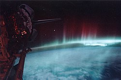
Earth's night-side upper atmosphere appearing from the bottom as bands of afterglow illuminating the troposphere in orange with silhouettes of clouds, and the stratosphere in white and blue. Next the mesosphere (pink area) extends to the orange and faintly green line of the lowest airglow, at about one hundred kilometers at the edge of space and the lower edge of the thermosphere (invisible). Continuing with green and red bands of aurorae streching over several hundred kilometers.

A diagram of the layers of Earth's atmosphere

The thermosphere is the layer in the Earth's atmosphere directly above the mesosphere and below the exosphere. Within this layer of the atmosphere, ultraviolet radiation causes photoionization/photodissociation of molecules, creating ions; the thermosphere thus constitutes the larger part of the ionosphere. Taking its name from the Greek θερμός (pronounced thermos) meaning heat, the thermosphere begins at about 80 km (50 mi) above sea level. ^[1] At these high altitudes, the residual atmospheric gases sort into strata according to molecular mass (see turbosphere). Thermospheric temperatures increase with altitude due to absorption of highly energetic solar radiation. Temperatures are highly dependent on solar activity, and can rise to 2,000 °C (3,630 °F) or more. Radiation causes the atmospheric particles in this layer to become electrically charged, enabling radio waves to be refracted and thus be received beyond the horizon. In the exosphere, beginning at about 600 km (375 mi) above sea level, the atmosphere turns into space, although, by the judging criteria set for the definition of the Kármán line (100 km), most of the thermosphere is part of space. The border between the thermosphere and exosphere is known as the thermopause.

The highly attenuated gas in this layer can reach 2,500 °C (4,530 °F). Despite the high temperature, an observer or object will experience low temperatures in the thermosphere, because the extremely low density of the gas (practically a hard vacuum) is insufficient for the molecules to conduct heat. A normal thermometer will read significantly below 0 °C (32 °F), at least at night, because the energy lost by thermal radiation would exceed the energy acquired from the atmospheric gas by direct contact. In the anacoustic zone above 160 kilometres (99 mi), the density is so low that molecular interactions are too infrequent to permit the transmission of sound.

The dynamics of the thermosphere are dominated by atmospheric tides, which are driven predominantly by diurnal heating. Atmospheric waves dissipate above this level because of collisions between the neutral gas and the ionospheric plasma.

The thermosphere is uninhabited with the exception of the International Space Station, which orbits the Earth within the middle of the thermosphere between 408 and 410 kilometres (254 and 255 mi) and the Tiangong space station, which orbits between 340 and 450 kilometres (210 and 280 mi).

Neutral gas constituents

It is convenient to separate the atmospheric regions according to the two temperature minima at an altitude of about 12 kilometres (7.5 mi) (the tropopause) and at about 85 kilometres (53 mi) (the mesopause) (Figure 1). The thermosphere (or the upper atmosphere) is the height region above 85 kilometres (53 mi), while the region between the tropopause and the mesopause is the middle atmosphere (stratosphere and mesosphere) where absorption of solar UV radiation generates the temperature maximum near an altitude of 45 kilometres (28 mi) and causes the ozone layer.

Figure 1. Nomenclature of atmospheric regions based on the profiles of electric conductivity (left), temperature (middle), and electron number density in m (right)

The density of the Earth's atmosphere decreases nearly exponentially with altitude. The total mass of the atmosphere is M = ρ_A H  ≃ 1 kg/cm² within a column of one square centimeter above the ground (with ρ_A = 1.29 kg/m³ the atmospheric density on the ground at z = 0 m altitude, and H ≃ 8 km the average atmospheric scale height). Eighty percent of that mass is concentrated within the troposphere. The mass of the thermosphere above about 85 kilometres (53 mi) is only 0.002% of the total mass. Therefore, no significant energetic feedback from the thermosphere to the lower atmospheric regions can be expected.

Turbulence causes the air within the lower atmospheric regions below the turbopause at about 90 kilometres (56 mi) to be a mixture of gases that does not change its composition. Its mean molecular weight is 29 g/mol with molecular oxygen (O₂) and nitrogen (N₂) as the two dominant constituents. Above the turbopause, however, diffusive separation of the various constituents is significant, so that each constituent follows its barometric height structure with a scale height inversely proportional to its molecular weight. The lighter constituents atomic oxygen (O), helium (He), and hydrogen (H) successively dominate above an altitude of about 200 kilometres (124 mi) and vary with geographic location, time, and solar activity. The ratio N₂/O which is a measure of the electron density at the ionospheric F region is highly affected by these variations. ^[2] These changes follow from the diffusion of the minor constituents through the major gas component during dynamic processes.

The thermosphere contains an appreciable concentration of elemental sodium located in a 10-kilometre (6.2 mi) thick band that occurs at the edge of the mesosphere, 80 to 100 kilometres (50 to 62 mi) above Earth's surface. The sodium has an average concentration of 400,000 atoms per cubic centimeter. This band is regularly replenished by sodium sublimating from incoming meteors. Astronomers have begun using this sodium band to create "guide stars" as part of the optical correction process in producing ultra-sharp ground-based observations. ^[3]

Energy input

Energy budget

The thermospheric temperature can be determined from density observations as well as from direct satellite measurements. The temperature vs. altitude z in Fig. 1 can be simulated by the so-called Bates profile: ^[4]

(1)  ${\displaystyle T=T_{\infty }-(T_{\infty }-T_{0})e^{-s(z-z_{0})}}$

with T_∞ the exospheric temperature above about 400 km altitude, T_o = 355 K, and z_o = 120 km reference temperature and height, and s an empirical parameter depending on T_∞ and decreasing with T_∞. That formula is derived from a simple equation of heat conduction. One estimates a total heat input of q_o≃ 0.8 to 1.6 mW/m² above z_o = 120 km altitude. In order to obtain equilibrium conditions, that heat input q_o above z_o is lost to the lower atmospheric regions by heat conduction.

The exospheric temperature T_∞ is a fair measurement of the solar XUV radiation. Since solar radio emission F at 10.7  cm wavelength is a good indicator of solar activity, one can apply the empirical formula for quiet magnetospheric conditions. ^[5]

(2)  ${\displaystyle T_{\infty }\simeq 500+3.4F_{0}}$

with T_∞ in K, F_o in 10⁻² W m⁻² Hz⁻¹ (the Covington index) a value of F averaged over several solar cycles. The Covington index varies typically between 70 and 250 during a solar cycle, and never drops below about 50. Thus, T_∞ varies between about 740 and 1350 K. During very quiet magnetospheric conditions, the still continuously flowing magnetospheric energy input contributes by about 250  K to the residual temperature of 500  K in eq.(2). The rest of 250  K in eq.(2) can be attributed to atmospheric waves generated within the troposphere and dissipated within the lower thermosphere.

Solar XUV radiation

The solar X-ray and extreme ultraviolet radiation (XUV) at wavelengths < 170  nm is almost completely absorbed within the thermosphere. This radiation causes the various ionospheric layers as well as a temperature increase at these heights (Figure 1). While the solar visible light (380 to 780  nm) is nearly constant with the variability of not more than about 0.1% of the solar constant, ^[6] the solar XUV radiation is highly variable in time and space. For instance, X-ray bursts associated with solar flares can dramatically increase their intensity over preflare levels by many orders of magnitude over some time of tens of minutes. In the extreme ultraviolet, the Lyman α line at 121.6 nm represents an important source of ionization and dissociation at ionospheric D layer heights. ^[7] During quiet periods of solar activity, it alone contains more energy than the rest of the XUV spectrum. Quasi-periodic changes of the order of 100% or greater, with periods of 27 days and 11 years, belong to the prominent variations of solar XUV radiation. However, irregular fluctuations over all time scales are present all the time. ^[8] During the low solar activity, about half of the total energy input into the thermosphere is thought to be solar XUV radiation. That solar XUV energy input occurs only during daytime conditions, maximizing at the equator during equinox.

Solar wind

The second source of energy input into the thermosphere is solar wind energy which is transferred to the magnetosphere by mechanisms that are not well understood. One possible way to transfer energy is via a hydrodynamic dynamo process. Solar wind particles penetrate the polar regions of the magnetosphere where the geomagnetic field lines are essentially vertically directed. An electric field is generated, directed from dawn to dusk. Along the last closed geomagnetic field lines with their footpoints within the auroral zones, field-aligned electric currents can flow into the ionospheric dynamo region where they are closed by electric Pedersen and Hall currents. Ohmic losses of the Pedersen currents heat the lower thermosphere (see e.g., Magnetospheric electric convection field). Also, penetration of high energetic particles from the magnetosphere into the auroral regions enhance drastically the electric conductivity, further increasing the electric currents and thus Joule heating. During the quiet magnetospheric activity, the magnetosphere contributes perhaps by a quarter to the thermosphere's energy budget. ^[9] This is about 250  K of the exospheric temperature in eq.(2). During the very large activity, however, this heat input can increase substantially, by a factor of four or more. That solar wind input occurs mainly in the auroral regions during both day and night.

Atmospheric waves

Two kinds of large-scale atmospheric waves within the lower atmosphere exist: internal waves with finite vertical wavelengths which can transport wave energy upward, and external waves with infinitely large wavelengths that cannot transport wave energy. ^[10] Atmospheric gravity waves and most of the atmospheric tides generated within the troposphere belong to the internal waves. Their density amplitudes increase exponentially with height so that at the mesopause these waves become turbulent and their energy is dissipated (similar to breaking of ocean waves at the coast), thus contributing to the heating of the thermosphere by about 250  K in eq.(2). On the other hand, the fundamental diurnal tide labeled (1, −2) which is most efficiently excited by solar irradiance is an external wave and plays only a marginal role within the lower and middle atmosphere. However, at thermospheric altitudes, it becomes the predominant wave. It drives the electric Sq-current within the ionospheric dynamo region between about 100 and 200  km height.

Heating, predominately by tidal waves, occurs mainly at lower and middle latitudes. The variability of this heating depends on the meteorological conditions within the troposphere and middle atmosphere, and may not exceed about 50%.

Dynamics

Figure 2. Schematic meridian-height cross-section of circulation of (a) symmetric wind component (P₂ ), (b) of antisymmetric wind component (P₁ ), and (d) of symmetric diurnal wind component (P₁ ) at 3 h and 15 h local time. Upper right panel (c) shows the horizontal wind vectors of the diurnal component in the northern hemisphere depending on local time.

Within the thermosphere above an altitude of about 150 kilometres (93 mi), all atmospheric waves successively become external waves, and no significant vertical wave structure is visible. The atmospheric wave modes degenerate to the spherical functions P_n^m with m a meridional wave number and n the zonal wave number (m = 0: zonal mean flow; m = 1: diurnal tides; m = 2: semidiurnal tides; etc.). The thermosphere becomes a damped oscillator system with low-pass filter characteristics. This means that smaller-scale waves (greater numbers of (n,m)) and higher frequencies are suppressed in favor of large-scale waves and lower frequencies. If one considers very quiet magnetospheric disturbances and a constant mean exospheric temperature (averaged over the sphere), the observed temporal and spatial distribution of the exospheric temperature distribution can be described by a sum of spheric functions: ^[11]

(3)  ${\displaystyle T(\varphi ,\lambda ,t)=T_{\infty }\{1+\Delta T_{2}^{0}P_{2}^{0}(\varphi )+\Delta T_{1}^{0}P_{1}^{0}(\varphi )\cos[\omega _{a}(t-t_{a})]+\Delta T_{1}^{1}P_{1}^{1}(\varphi )\cos(\tau -\tau _{d})+\cdots \}}$

Here, it is φ latitude, λ longitude, and t time, ω_a the angular frequency of one year, ω_d the angular frequency of one solar day, and τ = ω_dt + λ the local time. t_a = June 21 is the date of northern summer solstice, and τ_d = 15:00 is the local time of maximum diurnal temperature.

The first term in (3) on the right is the global mean of the exospheric temperature (of the order of 1000  K). The second term [with P₂⁰ = 0.5(3 sin²(φ)−1)] represents the heat surplus at lower latitudes and a corresponding heat deficit at higher latitudes (Fig. 2a). A thermal wind system develops with the wind toward the poles in the upper level and winds away from the poles in the lower level. The coefficient ΔT₂⁰ ≈ 0.004 is small because Joule heating in the aurora regions compensates that heat surplus even during quiet magnetospheric conditions. During disturbed conditions, however, that term becomes dominant, changing sign so that now heat surplus is transported from the poles to the equator. The third term (with P₁⁰ = sin φ) represents heat surplus on the summer hemisphere and is responsible for the transport of excess heat from the summer into the winter hemisphere (Fig. 2b). Its relative amplitude is of the order ΔT₁⁰ ≃ 0.13. The fourth term (with P₁¹(φ) = cos φ) is the dominant diurnal wave (the tidal mode (1,−2)). It is responsible for the transport of excess heat from the daytime hemisphere into the nighttime hemisphere (Fig. 2d). Its relative amplitude is ΔT₁¹≃ 0.15, thus on the order of 150 K. Additional terms (e.g., semiannual, semidiurnal terms, and higher-order terms) must be added to eq.(3). However, they are of minor importance. Corresponding sums can be developed for density, pressure, and the various gas constituents. ^{[5] [12]}

Thermospheric storms

In contrast to solar XUV radiation, magnetospheric disturbances, indicated on the ground by geomagnetic variations, show an unpredictable impulsive character, from short periodic disturbances of the order of hours to long-standing giant storms of several days' duration. The reaction of the thermosphere to a large magnetospheric storm is called a thermospheric storm. Since the heat input into the thermosphere occurs at high latitudes (mainly into the auroral regions), the heat transport is represented by the term P₂⁰ in eq.(3) is reversed. Also, due to the impulsive form of the disturbance, higher-order terms are generated which, however, possess short decay times and thus quickly disappear. The sum of these modes determines the "travel time" of the disturbance to the lower latitudes, and thus the response time of the thermosphere with respect to the magnetospheric disturbance. Important for the development of an ionospheric storm is the increase of the ratio N₂/O during a thermospheric storm at middle and higher latitude. ^[13] An increase of N₂ increases the loss process of the ionospheric plasma and causes therefore a decrease of the electron density within the ionospheric F-layer (negative ionospheric storm).

Climate change

A contraction of the thermosphere has been observed as a possible result in part due to increased carbon dioxide concentrations, the strongest cooling and contraction occurring in that layer during solar minimum. The most recent contraction in 2008–2009 was the largest such since at least 1967. ^{[14] [15] [16]}

See also

• Aerial perspective
• Aeronomy
• Air (classical element)
• Air glow
• Airshed
• Atmospheric dispersion modeling
• Atmospheric electricity
• Atmospheric Radiation Measurement Climate Research Facility (ARM) (in the U.S.)
• Atmospheric stratification
• Biosphere
• Climate system
  • Earth's energy budget
• COSPAR international reference atmosphere (CIRA)
• Environmental impact of aviation
• Global dimming
• Historical temperature record
• Ionosphere
• Hydrosphere
• Hypermobility (travel)
• Kyoto Protocol
• Leaching (agriculture)
• Lithosphere
• Reference atmospheric model

References

1. Duxbury & Duxbury (1997). Introduction to the World's Oceans (5th ed.).
2. Prölss, G.W., and M. K. Bird, "Physics of the Earth's Space Environment", Springer Verlag, Heidelberg, 2010
3. "Martin Enderlein et al., ESO's Very Large Telescope sees four times first light, Laser Focus World, July 2016, pp. 22-24".
4. Rawer, K., Modelling of neutral and ionized atmospheres, in Flügge, S. (ed): Encycl. Phys., 49/7, Springer Verlag, Heidelberg, 223
5. Hedin, A.E., A revised thermospheric model based on the mass spectrometer and incoherent scatter data: MSIS-83 J. Geophys. Res., 88, 10170, 1983
6. Willson, R.C., Measurements of the solar total irradiance and its variability, Space Sci. Rev., 38, 203, 1984
7. Brasseur, G., and S. Salomon, "Aeronomy of the Middle Atmosphere", Reidel Pub., Dordrecht, 1984
8. Schmidtke, G., Modelling of the solar radiation for aeronomical applications, in Flügge, S. (ed), Encycl. Phys. 49/7, Springer Verlag, Heidelberg, 1
9. Knipp, D.J., W.K. Tobiska, and B.A. Emery, Direct and indirect thermospheric heating source for solar cycles, Solar Phys., 224, 2506, 2004
10. Volland, H., "Atmospheric Tidal and Planetary Waves", Kluwer, Dordrecht, 1988
11. Köhnlein, W., A model of thermospheric temperature and composition, Planet. Space Sci. 28, 225, 1980
12. von Zahn, U., et al., ESRO-4 model of global thermospheric composition and temperatures during low solar activity, Geophy. Res. Lett., 4, 33, 1977
13. Prölss, G.W., Density perturbations in the upper atmosphere caused by dissipation of solar wind energy, Surv. Geophys., 32, 101, 2011
14. Science News, NASA (2010-07-15). "A Puzzling Collapse of Earth's Upper Atmosphere". National Aeronautics and Space Administration - Science News. Retrieved 2010-07-16.
15. Ho, Derrick (2010-07-17). "Scientists baffled by unusual upper atmosphere shrinkage". Cable News Network. Retrieved 2010-07-18.
16. Saunders, Arrun; Swinerd, Graham G.; Lewis, Hugh G. (2009). "Preliminary Results to Support Evidence of Thermospheric Contraction" (PDF). Advanced Maui Optical and Space Surveillance Technologies Conference: 8. Bibcode:2009amos.confE..55S. Archived (PDF) from the original on 2011-07-07.